Introduction

Continual learning is the project of training models on the data they generate in production. The model improves from real use rather than from curated approximations of use.

The setting is constrained in ways that benchmark training is not. Production gives one trajectory per user query, and those trajectories arrive at the trainer asynchronously, after the model has continued to update. Two properties follow for continual learning:

• Single rollouts. Each user query is drawn once. Methods that require multiple rollouts per task must synthesize the missing ones in a simulated environment, which is no longer the environment the model is deployed in.

• Off-policy data. By the time a trajectory reaches the trainer, the model has updated on earlier completions. The rollout was generated by an older policy, and any method that assumes otherwise degrades on stale data.

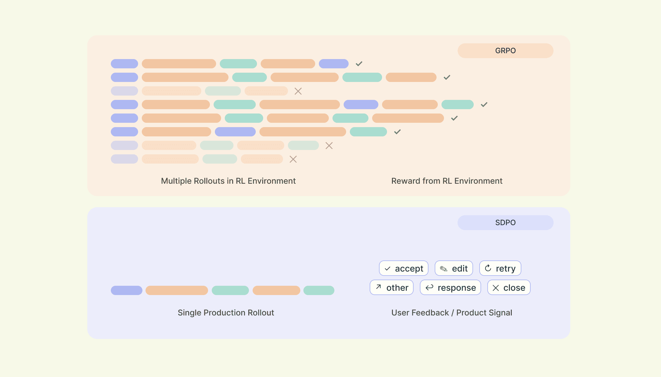
The dominant post-training method, GRPO, samples a group of rollouts on the same task, scores each one with a verifier, and updates the policy toward the relative rankings within the group. This works on benchmarks, where the same task can be sampled repeatedly. It also handles off-policy data through standard importance sampling and clipping. But it is fundamentally a group algorithm: with one rollout per task, the within-group ranking is undefined.

Self-Distillation Policy Optimization (SDPO), from Hübotter et al. [^1], is a leading candidate for the continual learning setting. The model is its own teacher: at each token of a rollout, the policy with no hint is updated to match the policy with a hint, where the hint is something the model could not have seen at rollout time but that retroactively reveals the right answer.

SDPO trains on a single trajectory, with no group required, and produces a gradient at every token rather than a scalar at the end. But every published SDPO result [^1][^2][^7] assumes the rollout was sampled from the current policy. Off-policy data breaks the recipe.

This post extends SDPO to off-policy data, which is the missing piece to using it for continual learning.

How SDPO works

SDPO, introduced by Hübotter et al. [^3], is a distillation method in which the model being trained is its own teacher. Given a prompt $s$, the student is the policy $π_θ(·|s)$ that we are training. The teacher is the same policy conditioned on a hint $c$, written $π_θ(·|s, c)$. The hint is privileged context that was not available to the student at rollout time but, in hindsight, would have helped: a successful sibling rollout [^3], the canonical answer [^7], or feedback from a user [^1].

The construction is three steps.

First, roll out the student on a task, producing a trajectory $τ = (s_1, a_1, ..., s_T, a_T)$ drawn from $π_θ$. Second, form the hinted distribution $π_θ(·|s_t, c)$ at each state $s_t$ by re-running the same weights with the hint $c$ prepended to the context. Third, train the student to match the hinted distribution at every position of $τ$.

There is no separate teacher model, no reward model, no human labels. The student and the hinted teacher are the same weights; the only difference is what each one sees.

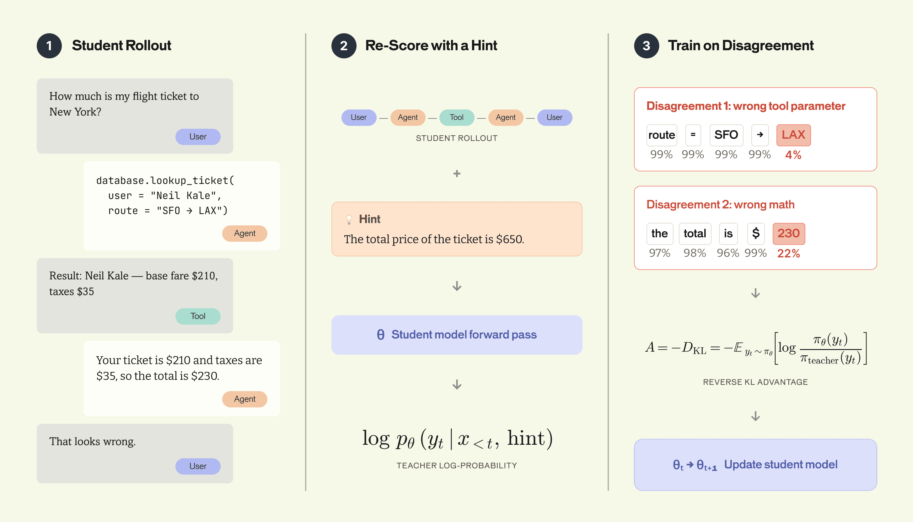
The loss is the per-token reverse KL between the student and the hinted teacher, summed over the trajectory:

$$\mathcal{L}_{\text{SDPO}}(\theta)=\mathbb{E}_{\tau\sim\pi_\theta}\left[\sum_{t=1}^T \text{KL}(\pi_\theta(\cdot|s_t)||\pi_\theta(\cdot|s_t,c))\right]$$

Reverse KL is mode-seeking: it pushes the student toward the hinted teacher's high-probability tokens rather than spreading mass across the full distribution, and when the student matches the teacher, the loss is zero. In practice we use the sampled-token form, sampling a token from the student, scoring with the teacher log-prob on that token, and updating the student toward/away from it. This is an unbiased estimator of the full KL.

SDPO's loss is defined per trajectory and per token. There is no group, no end-of-episode collapse, no separate reward model. This is the shape we need to investigate and confirm to truly train on production.

Experiment setup

We evaluate whether SDPO can learn in the production-shaped regime: one rollout per task, failures retained, and off-policy training.

We use two benchmarks. The first one is a modified version of Tau [^8] a multi-turn tool-use environment with customer-service-style tasks. We use Tau-Retail with Qwen-3-4B to test whether the basic SDPO recipe works. We then scale up to APEX-Agents, our target benchmark. It is Mercor's long-horizon agentic benchmark built around professional tasks with real-world economic value [^9]. It has much longer trajectories, lower pass rates, and substantially higher rollout cost. We use APEX-Agents with GPT-OSS-120B to test whether the recipe transfers to the regime we actually care about.

The promise of group size 1

For production learning, group size 1 is the critical case. A real user request produces one trajectory. If an algorithm needs several rollouts from the same task, those rollouts have to be manufactured in a simulator, which means we are no longer training directly on production data.

However, SDPO doesn't need group-relative advantage. Its loss is well-defined for a single trajectory regardless of whether it succeeded, so failed trajectories still produce gradients. And it doesn't need groups at all: a single trajectory per task is enough, as noted by Zhao et al. [^7].

We ran SDPO on Tau-Retail for 50 steps at three configurations: group size 4 without failed rollouts, group size 4 with failed rollouts, and group size 1 with failed rollouts.

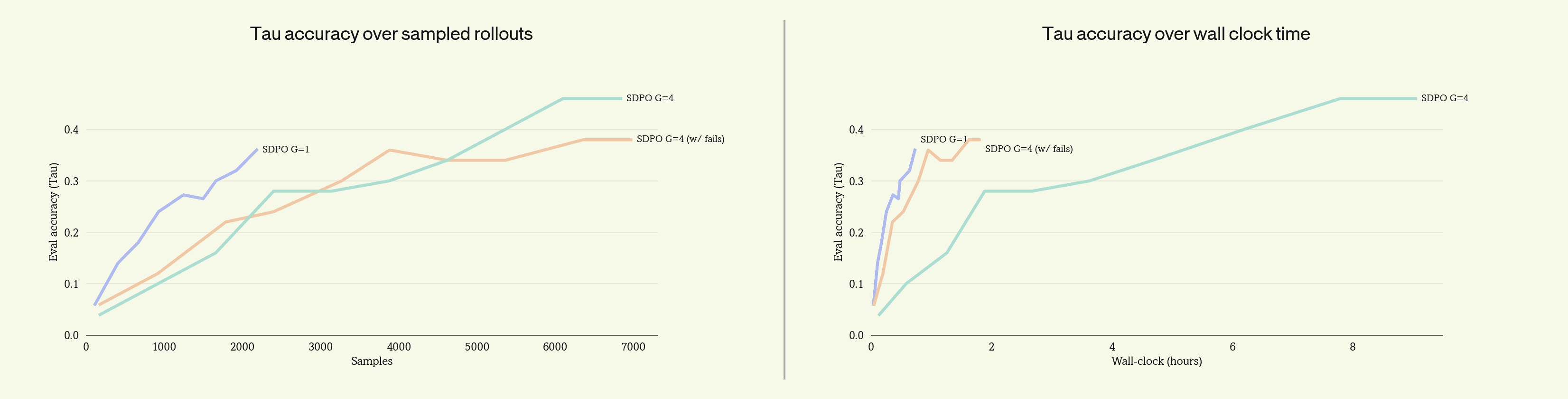
$G=1$ with failures retained is the most efficient configuration on both axes. Keeping failures at $G=4$ recovers most of the wall-clock gain, but reducing to $G=1$ unlocks the sample efficiency.

The shape of SDPO and the shape of production data line up: production gives one trajectory per user, SDPO learns from one trajectory per task. Both fall out of dropping group-relative advantage. The remaining question is whether SDPO can handle production's other defining property: that the data arrives off-policy.

The search for off-policy SDPO

Production data is off-policy. A user issues a query, the model responds, the trace eventually lands in the training queue, and by then the trainer has updated on whatever finished earlier; the policy that produced the rollout is not the policy being trained. Making the trainer wait for in-flight rollouts before stepping doesn't fix this, since it leaves the trainer idle for as long as the slowest user takes and the policy still moves on whatever has completed in the meantime.

We call the distance between the rollout policy $π_{θ−K}$ and the current policy $π_θ$ the staleness $K$, measured in trainer steps. $K$ is not a hyperparameter we choose; it’s set by trajectory length, user behavior, and trainer throughput, and rollouts arrive with whatever $K$ they arrive with.

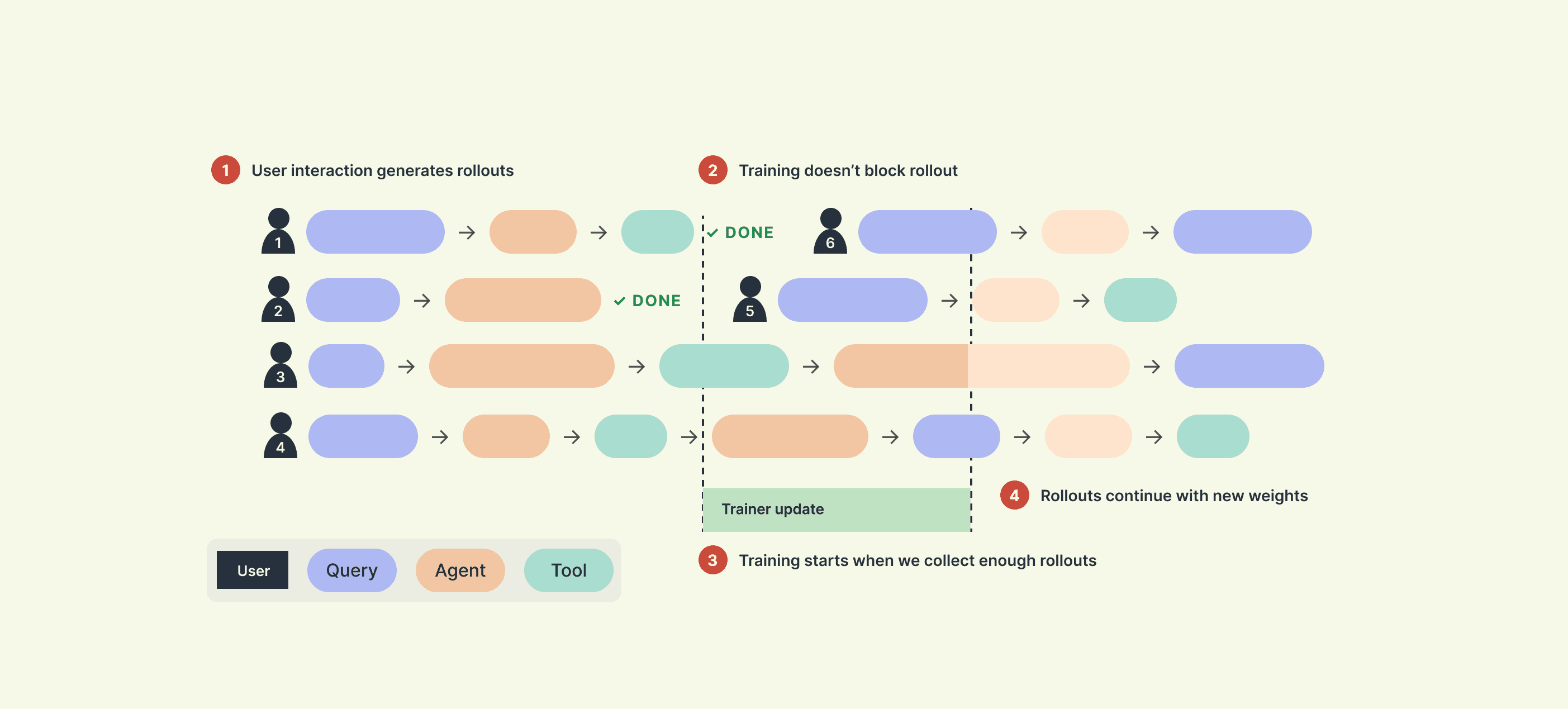
The same condition appears in any large-scale training run. Long-horizon rollouts vary in length by more than an order of magnitude — a single APEX trajectory can run over an hour while shorter ones finish in seconds — so synchronous training pays the cost of the longest tail on every step. The standard fix is to decouple the two clocks: rollout workers stream completions into a shared store, and the trainer pulls batches on its own schedule. This makes $K > 0$ the rule for any training at scale.

The published SDPO recipe assumes $K = 0$. Every result in Hübotter et al., Buening et al., and Zhao et al. uses synchronous rollouts on the current policy. Production can't satisfy this, and neither can any training run long enough to need async rollouts. If SDPO is going to be used in either setting, the recipe has to work at $K > 0$.

Naive SDPO collapses off-policy

The natural starting point is importance sampling (IS). Off-policy policy gradient methods have used IS corrections since at least Precup et al. (2000) [^10] and they remain the default in modern actor-critic methods like V-trace [^11] and Retrace [^12]. Applied to SDPO, the correction reweights each token by the ratio of the current policy to the rollout policy:

$$r_t = \frac{\pi_t(a_t|s_t)}{\pi_{\theta-K}(a_t|s_t)}$$

In expectation, the gradient is unbiased. In practice, it collapses.

We ran SDPO with this correction on Tau-Retail at $K=3$, e.g., max steps off-policy set to 3.

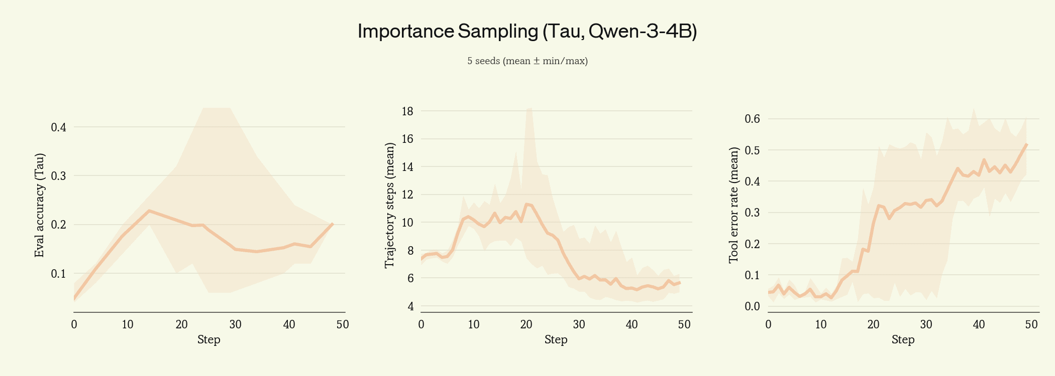
Training collapsed within fifty steps. The collapse mode points at the IS ratio. When the two policies are close, ratios cluster near 1 and the gradient estimator has bounded variance. When they diverge, the distribution of ratios becomes heavy-tailed: on rare tokens, where the rollout-time probability is small, the ratio can blow up to 50× or 100×, and a single such token can dominate the update.

This hurts SDPO more than it would hurt GRPO. GRPO's gradient is a single scalar advantage applied uniformly across the trajectory, so a blown-up ratio at one rare token gets averaged against the rest. SDPO has no such averaging: each token contributes its own KL, so a single position with an IS weight of 100 drives the whole update in its direction.

Starting from PPO

PPO's clip is the obvious place to start. It's the standard correction for unbounded importance-sampling ratios in policy gradient methods, and it shows up in GRPO, GSPO, and most of their cousins for exactly the failure mode we just saw. The ratio gets bounded to a fixed range around 1:

$$ r_t^{\text{clip}}=\text{clip}(r_t,1-\epsilon,1+\epsilon) $$

We reran the same experiment with PPO clipping at $ϵ=0.2$ and reran.

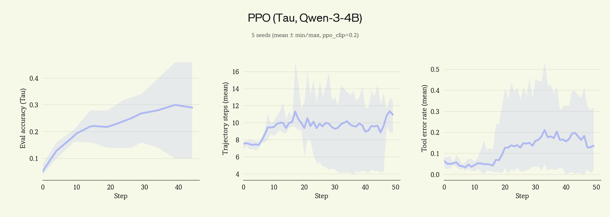
The collapse is gone, but the variance band on eval accuracy spans 0.10 to 0.45 at step 40. Same configuration, same hyperparameters, different seed, and the run can land anywhere in that range.

Clipping bounds the worst tokens but doesn't eliminate the problem it was solving. A clipped ratio of 1+ϵ is still a sizable update compared to a token at ratio 1, and a trajectory might contain dozens of clipped tokens. Which tokens get clipped depends on which rollouts a seed happens to sample, so different seeds end up applying different aggregated gradients to the same starting policy. Variance across seeds is the next problem to solve.

What about a KL penalty?

Two stabilizers are standard tools for variance reduction in policy gradient methods. A KL penalty to a reference policy, used throughout RLHF since Ziegler et al. [^13], bounds how far the policy can drift from a fixed anchor at every step. Per-token advantage clipping, from the original PPO work [^14], bounds the size of any individual token's contribution to the gradient. Both attack the seed-variance problem identified in the previous section, but through different mechanisms: KL penalty constrains the destination, advantage clipping constrains the step.

We ran both as ablations on top of PPO clipping.

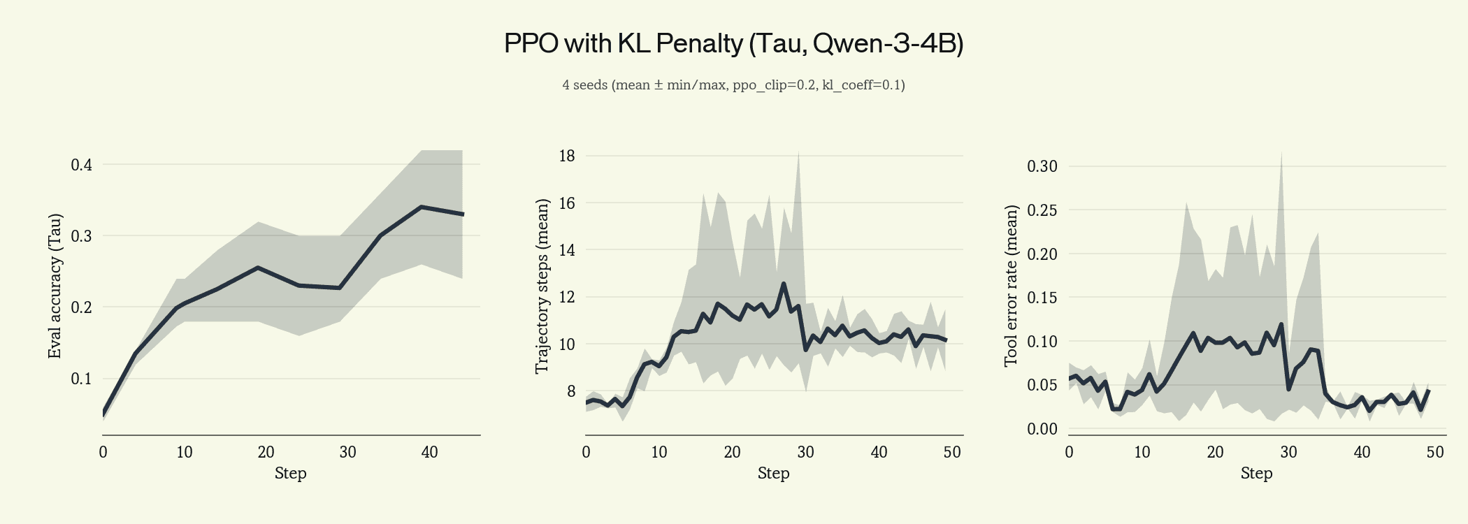
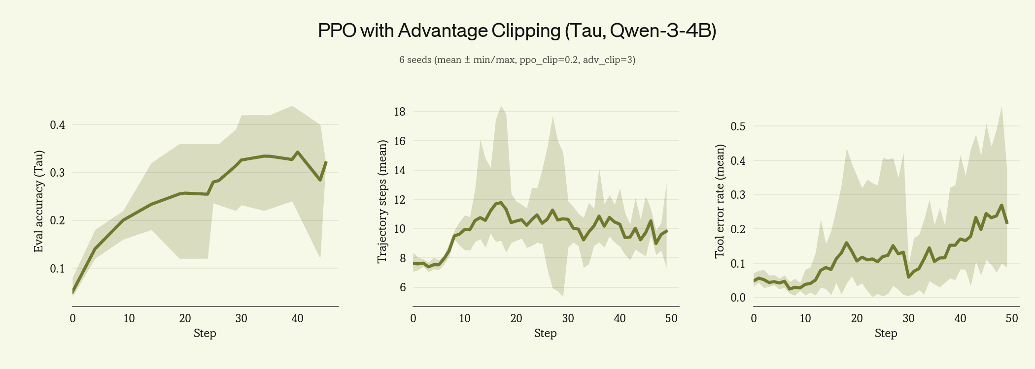
Both close the variance gap. KL penalty produces a slightly tighter eval accuracy band and lower tool error rate; advantage clipping shows more residual variance but reaches comparable mean accuracy.

We carry advantage clipping forward. The KL penalty requires running a reference model on every gradient step, roughly doubling the forward-pass compute, and it biases the policy toward whatever reference is chosen. Advantage clipping has neither cost: it bounds the per-token advantage at a fixed multiple of its running mean, discarding rare extreme updates without anchoring the policy to anything. We set the clip at 3× and use this for the rest of the post.

Scaling to APEX-Agents

Tau retail is a useful workbench, but it still falls short of representing a production agent’s rollouts. Mercor's APEX-Agents benchmark brings us a bit closer to the complexity often faced in production: rollouts run for an hour or more, the base pass rate is near zero, and most trajectories arrive as failures. We trained GPT-OSS-120B on APEX-Agents with the full configuration developed on Tau: PPO clipping at $ϵ=0.2$, advantage clipping at 3×, $K=3$, group size 1, all-fail groups retained.

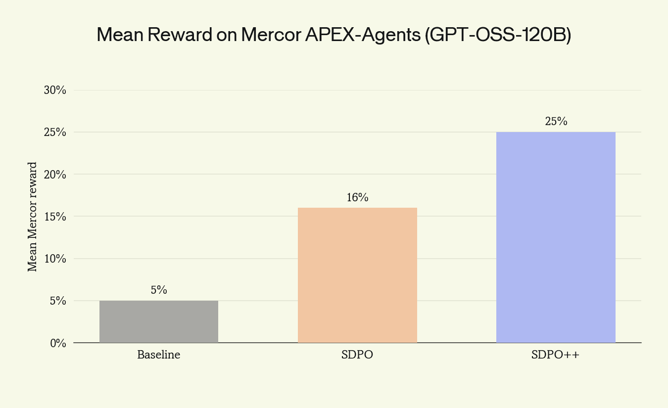
SDPO++ reaches 25% pass rate, a $5×$ improvement over the 5% zero-shot baseline and a 9-point gain over SDPO without the stabilizers. APEX-Agents has the four properties that define continual learning's regime: long rollouts, low base pass rate, stale data, single trajectories per task. Training runs stably under all of them at once, and produces a meaningful gain.

In Summary

For continual learning to actually work, production data has to be training data. Not data shaped like production, not synthetic approximations of production, but the trajectories that come out of users using the model. That is the regime SDPO turns out to be built for, almost by accident. Its loss is defined per trajectory, per token, without group-relative terms or end-of-episode collapse. Production gives one trajectory per user, arriving off-policy, with the user's behavior as the privileged context. The shapes match.

What we did in this post was make that match hold up. Group size 1 works in theory and in the runs. Off-policy training works once PPO clipping bounds the worst tokens and advantage clipping closes the seed variance. The result is an algorithm that does not need synchronous rollouts or fresh trajectories: production data, whenever it arrives and however stale, becomes usable training signal.

The APEX-Agents result is what makes this concrete. The same recipe developed on Qwen-3-4B at small scale carried over to GPT-OSS-120B on hour-long trajectories without retuning, producing a 5× improvement over zero-shot in a regime where GRPO's group filter would discard nearly every rollout. The algorithm runs where the previous approach could not start (without non-trivial reward shaping).

This opens up a training loop that runs on the user's clock, not the trainer's. The user acts, that becomes the hint, the model improves, the next user gets the better model. No environment construction, no per-customer verifier, no reward model. The signal is what the user actually did, and the algorithm consumes it directly.

What's still open

The stabilizers we landed on are empirical. PPO clipping bounds the rare-token blowups that crash naive off-policy SDPO, but it does not explain why SDPO is more sensitive to these blowups than other policy gradient methods. Advantage clipping closes the seed variance, but the 3× threshold is set by ablation, not derivation. There is a story to tell here about why SDPO's per-token KL responds the way it does to off-policy data, and we have not told it.

SDPO sharpens behaviors the model already has. The hinted teacher provides per-token targets for tokens the student already considers, but does not naturally guide the model toward behaviors it has not sampled. For hard tasks where the right behavior is rare in the base policy, secondary objectives like behavior cloning or DAgger may be needed. Our preliminary experiments in that direction showed enough hint-copying that hint design looks like the harder problem.

Soon, we will be running off-policy SDPO on live production traces, with the user's actual interactions as the hint. That is the regime this work was built for, and it is where we expect the remaining open questions to either resolve or sharpen.

Acknowledgements

We’d like to thank Dian Ang Yap, Michael Elabd, Jerry Chan, and Chuck Tang for their contributions to the technical portions of this blog post.

Thanks also to Arjun Karanam, Irene Han, Ronak Malde, Albert Li, and Hersh Godse for their contributions to writing and artifact creation, and to Jennifer Zhai for her team coordination.

Citations

[^1]: Buening, T. K., Hübotter, J., Pásztor, B., Shenfeld, I., Ramponi, G., & Krause, A. (2026). Aligning language models from user interactions. arXiv preprint arXiv:2603.12273.

[^2]: Chakraborty, Souradip and Ziems, Noah and Huang, Furong and Jiang, Meng and Bedi, Amrit Singh and Khattab, Omar, "Pedagogical RL: Teaching Models to Teach Themselves from Privileged Information", 2026.

[^3]: Hübotter, J., Lübeck, F., Behric, L., Baumann, A., Bagatella, M., Marta, D., ... & Krause, A. (2026). Reinforcement Learning via Self-Distillation. arXiv preprint arXiv:2601.20802.

[^4]: Lu, Kevin and Thinking Machines Lab, "On-Policy Distillation", Thinking Machines Lab: Connectionism, Oct 2025.

[^5]: Mnih, V., Badia, A. P., Mirza, M., Graves, A., Lillicrap, T., Harley, T., ... & Kavukcuoglu, K. (2016, June). Asynchronous methods for deep reinforcement learning. In International conference on machine learning (pp. 1928-1937). PmLR.

[^6]: Shao, Z., Wang, P., Zhu, Q., Xu, R., Song, J., Bi, X., ... & Guo, D. (2024). Deepseekmath: Pushing the limits of mathematical reasoning in open language models. arXiv preprint arXiv:2402.03300.

[^7]: Zhao, S., Xie, Z., Liu, M., Huang, J., Pang, G., Chen, F., & Grover, A. (2026). Self-Distilled Reasoner: On-Policy Self-Distillation for Large Language Models. arXiv preprint arXiv:2601.18734.

[^8]: Yao, S., Shinn, N., Razavi, P., & Narasimhan, K. (2024). $\tau $-bench: A Benchmark for Tool-Agent-User Interaction in Real-World Domains. arXiv preprint arXiv:2406.12045.

[^9]: Vidgen, B., Fennelly, A., Pinnix, E., Benchek, J., Khan, D., Richards, Z., ... & Nitski, O. (2025). The ai productivity index (apex). arXiv preprint arXiv:2509.25721.

[^10]: Precup, D., Sutton, R. S., & Singh, S. (2000). Eligibility traces for off-policy policy evaluation.

[^11]: Espeholt, L., Soyer, H., Munos, R., Simonyan, K., Mnih, V., Ward, T., ... & Kavukcuoglu, K. (2018, July). Impala: Scalable distributed deep-rl with importance weighted actor-learner architectures. In International conference on machine learning (pp. 1407-1416). PMLR.

[^12]: Munos, R., Stepleton, T., Harutyunyan, A., & Bellemare, M. (2016). Safe and efficient off-policy reinforcement learning. Advances in neural information processing systems, 29.

[^13]: Ziegler, D. M., Stiennon, N., Wu, J., Brown, T. B., Radford, A., Amodei, D., ... & Irving, G. (2019). Fine-tuning language models from human preferences. arXiv preprint arXiv:1909.08593.

[^14]: Schulman, J., Wolski, F., Dhariwal, P., Radford, A., & Klimov, O. (2017). Proximal policy optimization algorithms. arXiv preprint arXiv:1707.06347.

Appendix: How far can we push staleness?

By the time a long rollout lands in the store, the trainer may have taken several gradient steps on shorter rollouts that finished earlier. The policy that generated the rollout, $π_{\theta - K}$, is no longer the policy being trained, $π_\theta$. We call the distance $K$ the staleness.

In our main post, we fix staleness to 3 steps. To motivate that, note that higher staleness means the trainer waits less, runs at higher utilization, and converges faster in wall-clock time. But it also means a wider gap between rollout-time and current policy, which PPO clipping has to bridge through harder and harder cases. At some point the clipping stops being enough.

We ran a staleness sweep on Tau retail no-user from $K = 0$ to $K = 10$, measuring final accuracy and wall-clock time to convergence at each setting.

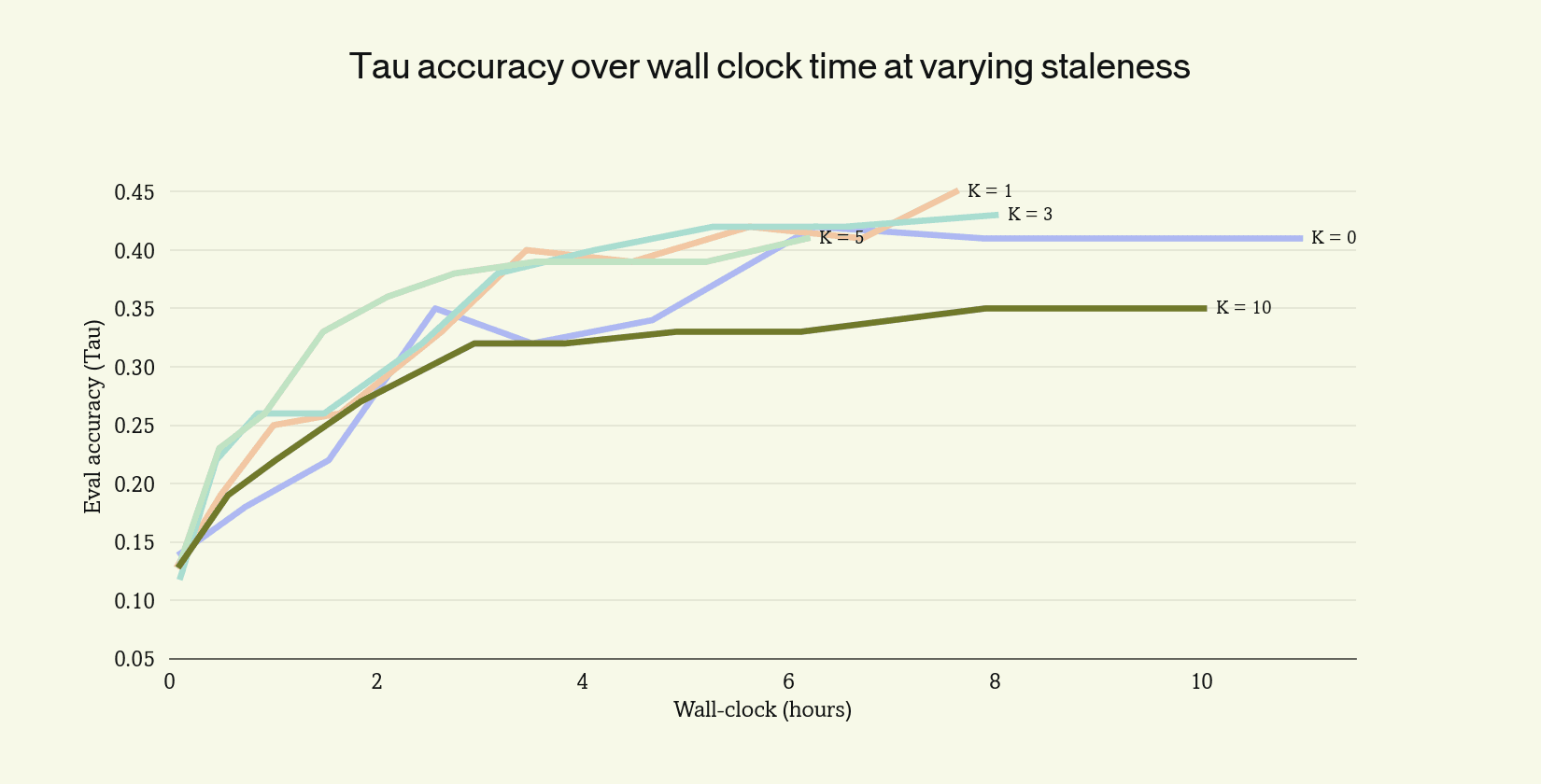
Accuracy is flat within noise from $K = 0$ up through $K = 3$, then begins to degrade. The right operating point is the largest $K$ at which accuracy is still preserved. For Tau retail no-user that is $K = 3$, where we get $2×$ wall-clock speedup over the synchronous baseline with no loss of final accuracy.