


The hardest part of training your own model is defining what good looks like.
For coding agents, we can use unit tests to check whether a solution works. But for tasks like legal analysis, investment banking, or customer support, there isn't always a clear right answer. Oftentimes, it comes down to expert judgment, and standards differ from company to company.
To train a model using reinforcement learning, we need to turn these standards into a reward function, something that can evaluate the model’s quality of output and steer it in the right direction.
The problem is that writing these reward functions is extremely time intensive. An entire training run requires thousands of tasks, and the experts best equipped to label these tasks can’t realistically write a rubric for every one.
So what if we could learn how an expert grades from just a few examples, and use that to extrapolate to thousands of new tasks?
We introduce Continual Grading, a way to do exactly this. By providing a small set of expert examples, we can learn a metagrader that generates grading criteria for tasks it hasn't seen before.
Instead of needing experts to define what good looks like for every task, we can learn from their taste and extend it to new data, continually improving the grading system as more feedback comes in.
The grading problem
To train a model with reinforcement learning, we need a reward function . Given a task and the model’s response , it returns a score for how good the response is. Training then pushes the model toward behaviors where responses score higher.
The big bottleneck is that someone has to write that reward function for every task. For coding, that usually means unit tests, which are easier for engineers to write. But for a merger memo, it means a lawyer deciding which protections the memo needs, and requires a lot of manual work. And invariably, a model needs thousands of tasks in order to train. At 30 minutes per task, 10,000 tasks comes out to 5,000 hours, about two and a half years of one expert’s time.
Also, the work also doesn’t stop once training starts. Production traffic keeps coming and the mix of tasks shifts, so the same criteria written in March may not be applicable for new data that comes in June.
Thus, a grading system for this setting needs to:
- learn what good looks like from a few expert examples
- tailor its grading to each task
- handle tasks no one has labeled
Existing approaches
There are a few common routes to grade rollouts that have no verifiable answer. Each approach holds a tradeoff between the manual effort required and the accuracy to true expert grading.
LLM judges
The simplest option is to have an LLM score each response (a generic LLM judge), or pick the better of two [Zheng et al., 2023]. This is quite cheap and broadly works on any task, since all it needs is a prompt.
The limitation though, is that the judge is limited by its own knowledge. The grades it outputs can only be as good as its understanding of the task, and in practice that ceiling is quite low. On hard examples where one answer is actually the correct one, research finds that strong LLM judges do only slightly better than random guessing [Tan et al., 2024].
Rubrics
A rubric gives the judge a way to judge against something concrete. Here, the model outputs a list of criteria for each task, and the judge checks each criteria separately. Rubrics are also easy to interpret. An expert can see which criteria a response missed and fix a bad criterion directly.
The catch, though, is that every task needs its own rubric, and writing thousands of them brings back the cost problem that we highlighted earlier. A logical fix is to have an LLM write the rubrics. This works well, as long as the LLM writing the rubric has a reference answer to work from [Gunjal et al., 2025].
Without a reference answer, the LLM is writing down its own idea of a good answer, so the rubric encounters the same ceiling as an LLM judge. And writing a reference answer for every task is valuable time from an expert, which is the cost we were trying to avoid in the first place.
Reward models
Judges and rubrics both depend on someone to write down what good looks like. A reward model offers another solution, which is to learn from a breadth of examples. As an input, experts label pairs of responses to the same task, marking the better one and the worse one .
The reward model is a network with weights shared across all tasks. Training pushes it to score above , using the Bradley-Terry loss [Bradley and Terry, 1952; Lambert, 2025]:
Because the weights are shared, one reward model can grade tasks it hasn’t seen. But learning a good set of weights means labelling thousands of labeled pairs, which is far more than the handful of examples we want to ask for.
A reward model is typically only accurate on responses like the ones it was trained on. During training, as RL improves the model, its responses drift away from that data. Eventually the model learns to exploit the reward model’s mistakes, and its reward goes up while the real quality goes down [Gao et al., 2022].
Learning a grader from labels
So far, each approach only satisfies part of our requirements. Judges and reward models work on any task, but a judge isn’t grounded in anything, and a reward model needs thousands of labels to work. Rubrics are grounded and readable, but requires someone to write one for every task.
What we want combines the best properties from each of these approaches. It should learn from a few labeled examples, tailor its grading to each task, and handle tasks no one has labeled. Inverse Constitutional AI comes the closest. It compresses a set of preferences into a short list of written principles, which a judge can then follow when grading new responses [Findeis et al., 2024].
The core limitation is that it learns from only one list of principles and applies it to every task. A list shared across all tasks can only hold what those tasks have in common, like general principles of good work. What makes a response good on one particular task might not necessarily fit, so for that part the judge falls back on its own knowledge, with the same ceiling as before.
| Learns from a few examples | Tailored to each task | Handles unseen tasks | |
|---|---|---|---|
| LLM judges | ✗ | ✗ | ✓ |
| Rubrics | ✗ | ✓ | ✗ |
| Reward models | ✗ | ✓ | ✓ |
| Inverse Constitutional AI | ✓ | ✗ | ✓ |
| Ideal solution | ✓ | ✓ | ✓ |
Every approach we have explored gives up something. Methods that handle new tasks either learn nothing from experts or they need thousands of labels, and the methods that learn from a few labels end up grading every task too uniformly. The ideal solution is a way to learn from a few expert examples just once, then use that to write a tailored grader for every incoming task.
Metagraders
We explore a way to address all three requirements for an ideal grader: one that learns from a few expert examples, tailors its grading to each task, and handles tasks no one has labeled.
What is a metagrader?
Recall that Inverse Constitutional AI learns a set of grading principles and applies them to every task. But even within law, different tasks need different criteria. The qualities to check for in a rental agreement aren’t necessarily the same things that make a correct merger agreement.
We take this one step further. Instead of learning a single grader, we learn a procedure that generates graders for new tasks. We call this procedure a metagrader.
A metagrader learns from a small set of expert-graded tasks. When it encounters a new task, it uses what it learned to construct a grader specifically for that task.
More formally, a metagrader is a program made up of prompts and code that uses a fixed judge model . Given a task , it produces a task-specific grader , which then assigns a score to a response .
This is essentially the same role a reward model plays. A reward model learns a set of weights that is learned across all tasks, where it sees pairs of responses where an expert preferred over [Bradley and Terry, 1952]:
A metagrader uses a similar objective, but we change what is actually learned. Instead of weights, we search over programs , where is the score that the grader writes for task gives to :
Like a reward model, a metagrader is also shared across tasks, and so it can also grade tasks it has never seen. The key difference is that what it learns is a readable program, so it is interpretable to an expert and can learn from a much smaller set of data.
This gives us the three properties we were looking for: it can learn from a small number of expert examples, produce different grading criteria for different tasks, and apply what it learned to tasks no expert has graded.
The idea of a metagrader builds on top of harness optimization, where we improve the prompts and code around a model rather than updating its weights [Zhang, 2026]. Methods like GEPA [Agrawal et al., 2025] and Meta-Harness [Lee et al., 2026] show how these programs can be optimized from a seed of relatively few examples, as it relies on the in-context learning capabilities of a model.
Learning a metagrader
We start with a small set of expert-graded tasks, which we use to learn and select a metagrader. We divide the data into four sets:
- : Expert-graded tasks used to build candidate metagraders.
- : Expert-graded tasks held out to select the best candidate.
- : Tasks used for the actual RL training, where the metagrader generates rewards without knowing the true expert graders.
- : Held-out expert-graded tasks used to evaluate the metagrader and the trained model.
We then use meta-harness search to learn a metagrader. A strong model, GPT-6-Astra Max, reads the tasks in , including their grading criteria, previous scores, and evaluator code. Then, the strong model generates several candidate metagraders, each with its own prompts and code.
Next, we use a simple best-of-N search to select the best candidate out of the ones generated. Each metagrader grades responses on , and we compare its own judgments against the expert graders. We select the candidate with the highest ranking accuracy, meaning that it most often agrees with the expert on which of two responses is better.
Once selected, the metagrader now generates graders for tasks in , which provide end rewards for RL. Finally, we use to measure how well the metagrader and the trained model perform on unseen tasks.
A nice property is that search doesn't need a differentiable loss, so in practice we replace the Bradley-Terry objective with ranking accuracy: the fraction of response pairs that the metagrader orders the same way as the expert [Lambert et al., 2024].
Ranking accuracy also works for pairwise graders, which only say which response is better. And it lines up with what RL needs. GRPO's gradient is essentially an average over pairwise comparisons between responses to the same task [Zhou et al., 2026], so that a grader that orders pairs correctly pushes training in roughly the right direction.
Metagrader designs
So far, we've described how to learn a metagrader, but there's still a choice in how it should grade responses. We explored three approaches, each building on the limitations of the previous one.
Scalar graders
The simplest approach is to have a judge model assign each response a score in .
In this case, the metagrader learns the prompts and checks used to produce that score. This is relatively cheap, since each response is graded on its own with a fixed number of judge calls.
For example, here is the scalar metagrader our search found on -Bench. Nobody specified this structure. The search arrived at it from the 30 graded tasks in : one call works out the task's core requirements and scores whether they're met, a second compares that score against the trajectory, and a third newly scores the response without seeing the first response. Then finally, the reward averages the last two together.
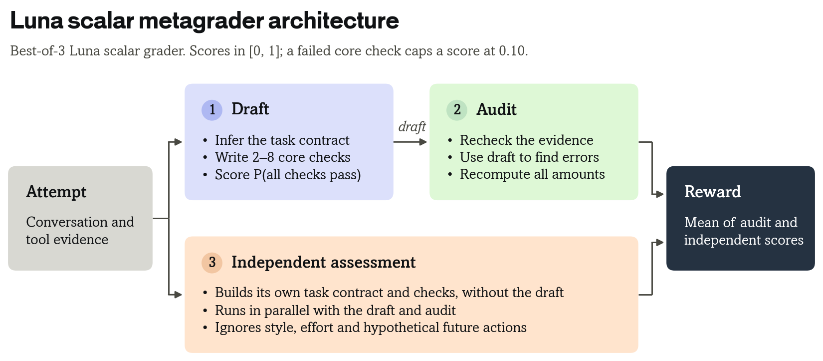
The main limitation is score calibration. A judge might give two responses similar scores even when one is significantly better. For RL, the primary thing we care about is whether the rewards reliably distinguish better responses from worse ones.
Pairwise graders
Instead of grading responses independently, we can ask the judge to compare two responses and have it select which one is better.
This achieves a nice property in that it avoids forcing the judge to assign absolute scores. Given a task and two responses and , the judge only needs to decide which response is better.
For a group of responses, we compare each response against the others, and we use the win rate as the reward:
This is quite analogous with GRPO, which learns from differences between responses to the same task.
The big downside for pairwise graders, however, is cost. Scalar grading requires evaluations for a group of responses, while pairwise grading requires directed comparisons if both orders are being evaluated.
More importantly, neither approach necessarily tells us why a response was good or bad. Even if a judge consistently prefers the better response, it may still be relying on its own judgment rather than the specific criteria that matter to the expert.
Rubric-based graders
This led us to a different approach: instead of asking the judge to directly score or compare responses, we have the metagrader first generate a rubric for each task.
A rubric contains criteria , each with a weight . A judge checks whether the response satisfies each criterion, and we combine the results into a single reward:
Unlike approaches that generate rubrics from reference answers [Gunjal et al., 2025], our metagrader learns how to construct them from the expert labels in .
The advantage to this approach is that the metagrader has to make its grading criteria explicit before evaluating the response. Rather than relying on a single overall judgment, it can check the specific factors that matter for the task.
This also makes the graders easier to inspect. An expert can see which criteria were met, identify mistakes, and correct individual criteria without rewriting the entire grader.
Results
We want to see if a model can be trained from graders built using a small number of expert examples, rather than needing expert-written graders for every training task.
We test this on two kinds of work: customer service and business workflows in -Bench [Yao et al., 2024; Barres et al., 2025], and legal analysis in Harvey-LAB [Grupen et al., 2026], and train Inkling Small 276B-A12B. Regardless of how a model is trained, we evaluate it against the original task graders for eval scores.
The main finding we care about is how much of the improvement from expert-written graders we can recover with a metagrader, without seeing these true graders.
A generic judge isn’t enough
The first approach we measured is the most basic alternative to expert grading: asking a general-purpose LLM to score each response it sees.
We ran this on -Bench, using GPT-6-Luna with a simple prompt asking it to assign a score from 0 to 1. We then trained against these scores for 40,000 rollouts, alongside a model trained on the original task graders.
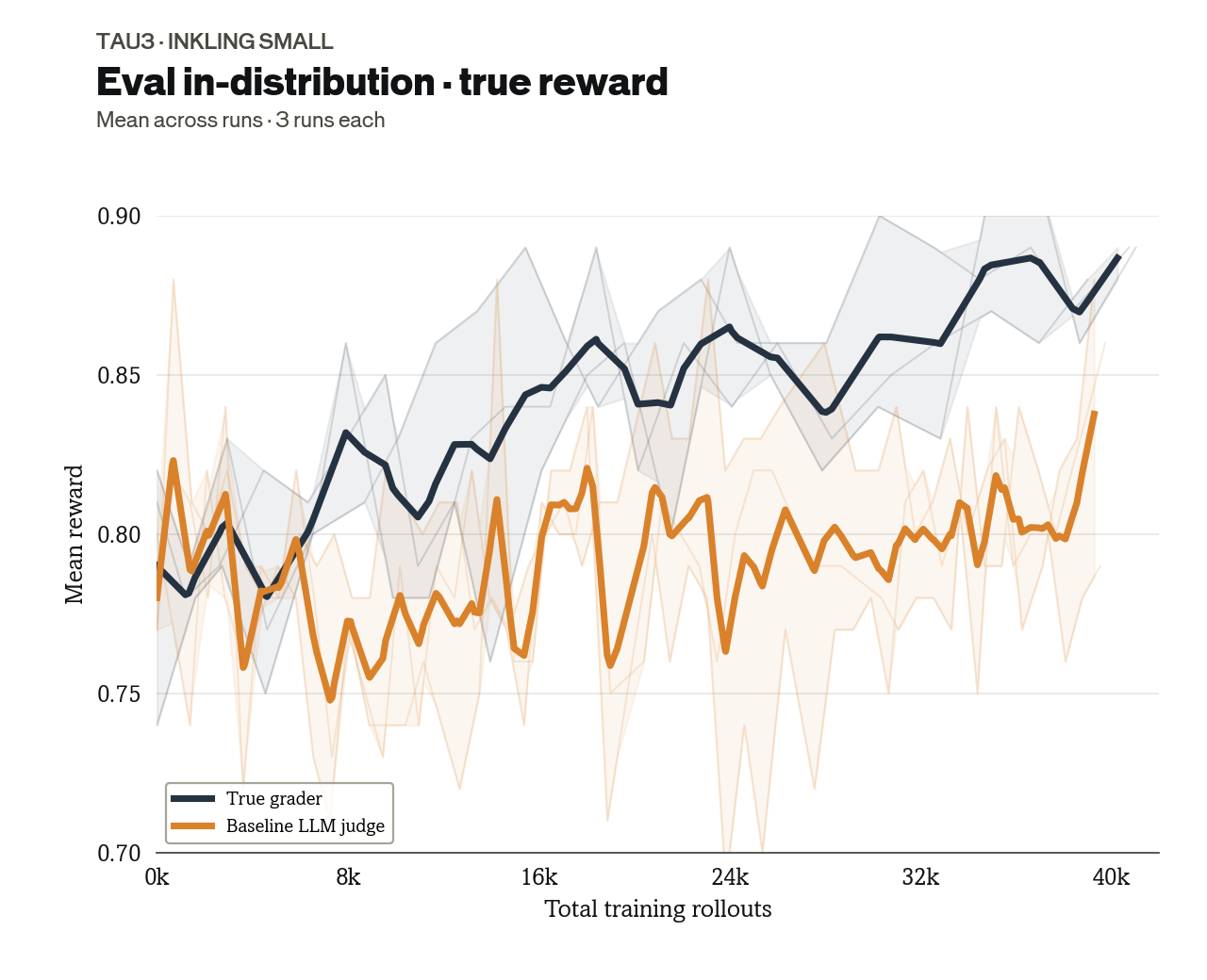
The model trained on the generic judge showed essentially no improvement, while the one trained on the original grader improved steadily.
This is a problem with using LLM judges out of the box. They can produce reasonable-looking scores for almost any response, but those scores don't necessarily reflect what the task actually requires, and training against them doesn't necessarily make the model better at the task.
Learning from a few expert examples
We next tried giving the judge examples of how experts actually grade.
On -Bench, we used 30 expert-graded tasks to construct candidate metagraders and another 30 to select the best one, for a total of 60 labeled tasks out of 375 in the benchmark.
We searched over scalar and pairwise metagraders, using Luna and Jev as the underlying judges, and we measured how well each agreed with the original graders before training.
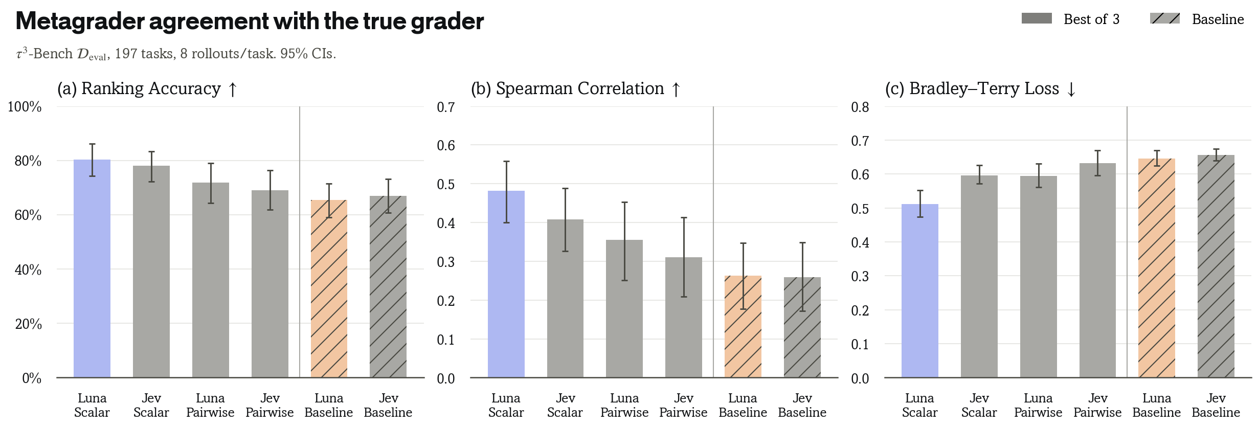
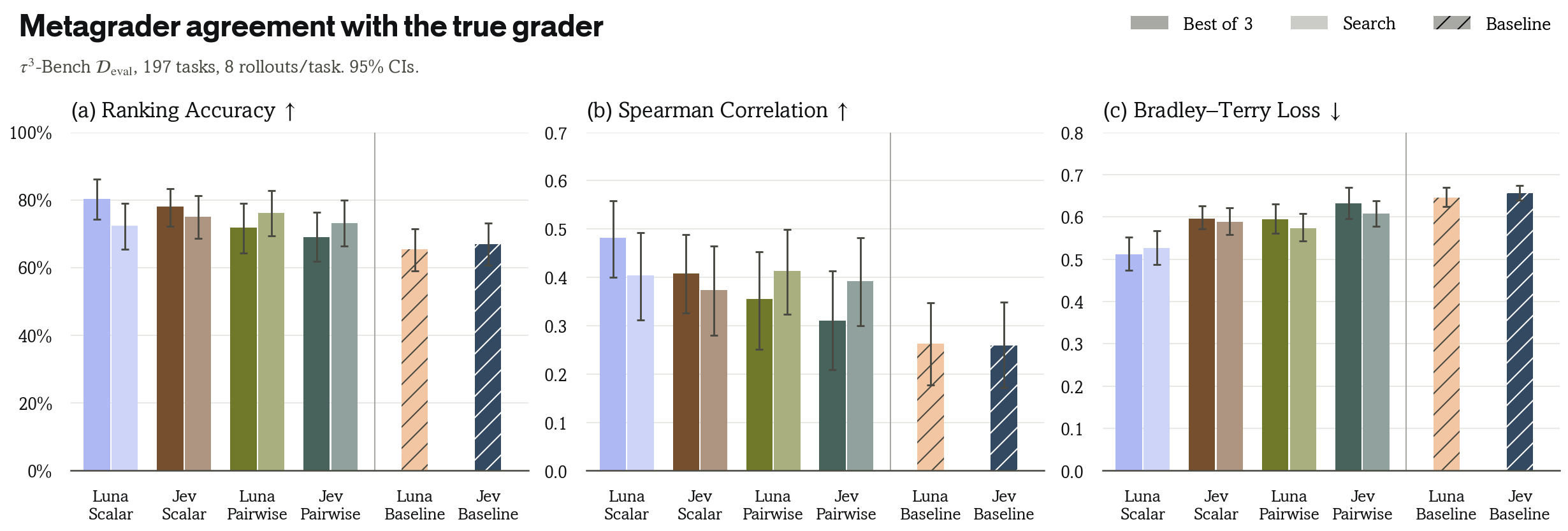
The scalar metagrader built with Luna performed the best, where it correctly ranked 80.3% of response pairs compared with 71.8% for the pairwise version. Pairwise grading was also more expensive because it required comparing responses against one another.
Then, we selected the scalar Luna metagrader and used its rewards to train Inkling Small with GSPO [Zheng et al., 2025]. We ran the same training with the original task graders as a comparison, using three seeds in each condition and ran evaluations for both on held-out tasks.
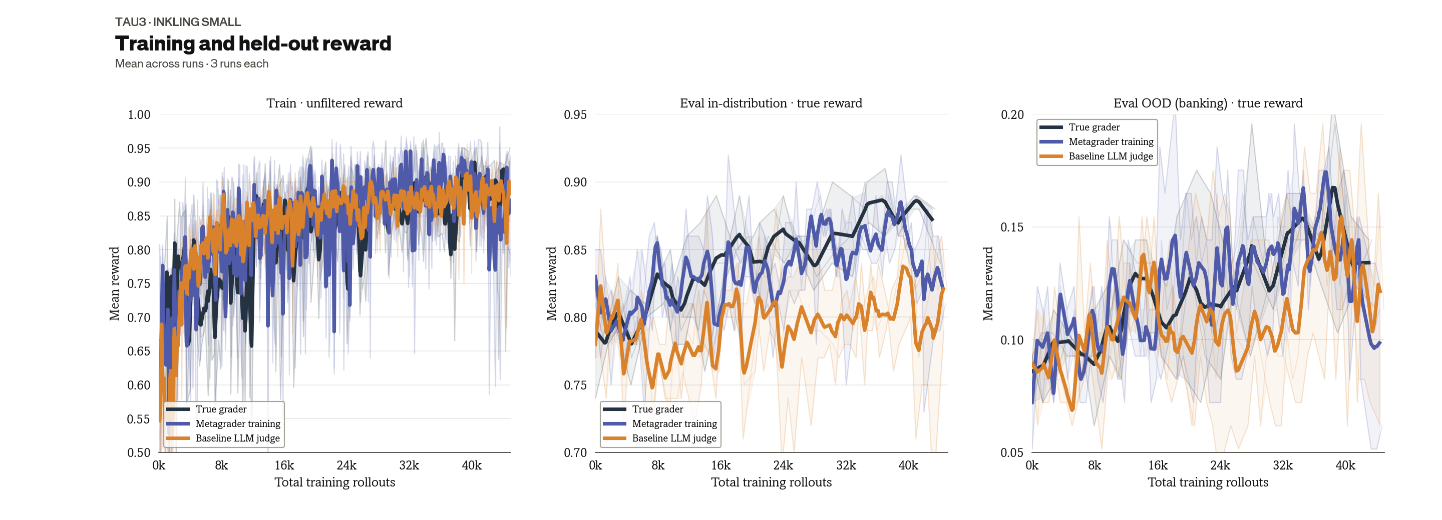
The model trained on the metagrader improved from 80.0% to 84.9%, compared with 87.8% when trained on the original grader.
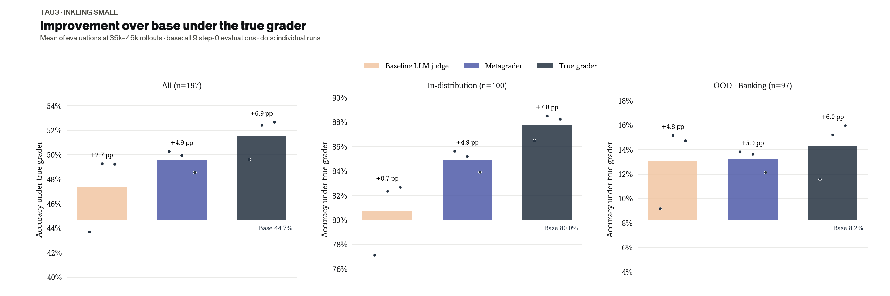
We also held out the entire banking domain while building and selecting the metagrader, to see whether it could grade work from a domain where it hadn't seen any expert examples.
On banking tasks, the metagrader-trained model improved from 8.2% to 13.2%, compared with 14.3% for the model trained on the original grader.
With just 60 labeled tasks, we are able to recover much of the improvement from expert grading, including on a domain the metagrader hadn't been trained to grade.
When a single score isn't enough
Scalar grading worked well on -Bench, but we found it struggled with legal work, where a response can be partially correct while still missing several important details.
Harvey-LAB contains 2,010 legal tasks, each evaluated against expert-written pass/fail criteria. For these experiments, we used 48 labeled tasks to construct metagraders and another 48 to select them, sampling across different legal practice areas.
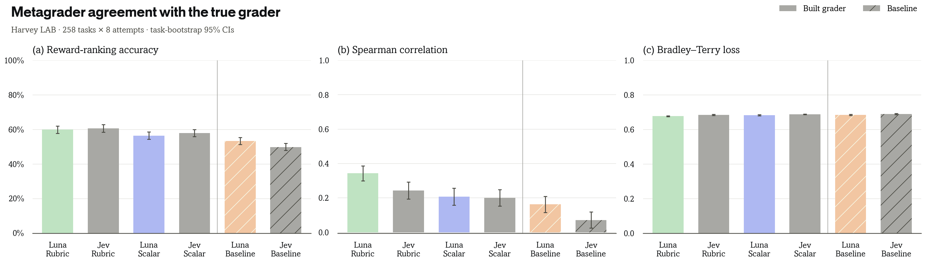
Ranking accuracy for scalar grading dropped from around 80% on -Bench to below 60% on Harvey-LAB, with either underlying judge.
Some of this comes from the difficulty of legal grading itself, since Harvey's expert judge only agrees with itself about 86% of the time. But looking at eight attempts on the same task (Figure 10), we can also see that the scalar grader gives similar scores to memos that are different on specific requirements, such as a missing clause or an incorrect citation.
We then tried to have the metagrader generate a rubric for each task, so that instead of assigning one overall score, it checks each requirement separately.
This improved agreement with the expert grader. Using Luna, Spearman correlation increased from 0.21 to 0.34, while ranking accuracy also improved by about four percentage points.
The grader-selection procedures weren't identical, so we can't attribute the entire difference to the rubric format. Still, for tasks where quality depends on many specific requirements, checking those requirements individually seems to give us a better grading signal.
Training with synthetic rubrics
The real test is training. We trained Qwen3.6-35B-A3B on Harvey-LAB using either the metagrader's generated rubrics or the original expert-written rubrics, with three seeds for each setting.
For evaluation, we use all-pass, the percentage of tasks where a response satisfies every criterion in the expert rubric. This is a pretty strict metric, since missing even one requirement means the task doesn't count as passed.
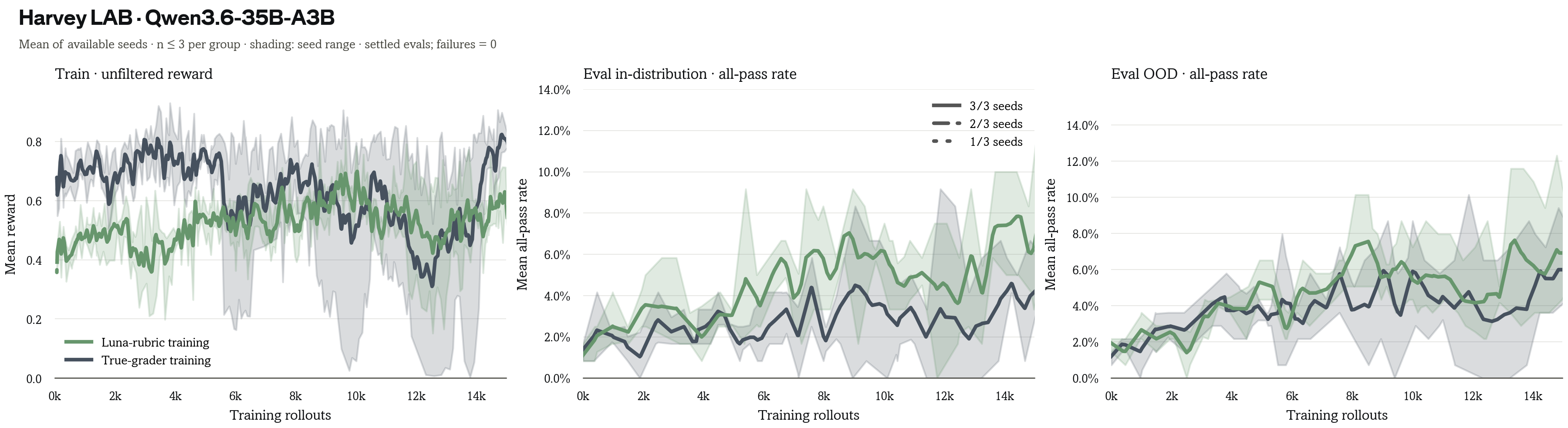
Across evaluations at 12,500–17,500 training rollouts, the model trained on generated rubrics averaged 6.6% all-pass, compared with 4.4% for the model trained on expert rubrics. Both started at 1.4%.
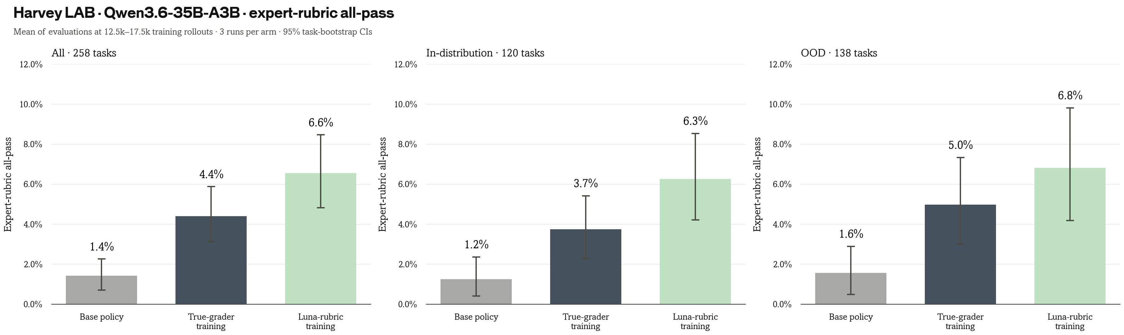
The confidence intervals overlap, so we can't conclude that generated rubrics perform better, although both approaches clearly improve over the starting model.
With 48 expert-labeled tasks for construction and another 48 for selection, the metagrader produced rubrics that trained the model comparably to expert-written rubrics for every task. This suggests we can reduce the amount of expert grading required to train on new tasks.
Analysis and discussion
Measuring a metagrader without training
Training a policy is expensive, so we'd like to know whether a metagrader is useful before spending compute on RL. We do this by generating eight rollouts per each held-out task using the base model, and then comparing the metagrader's scores against the original grader.
The core assumption is that a metagrader that agrees with the true grader on these initial rollouts is more likely to provide useful rewards during training. This isn't guaranteed, since the policy will change as it trains, but it at least gives us a practical way to select between candidate metagraders before training.
We measure agreement in three ways.
Ranking accuracy measures how often the metagrader is able to correctly identify which of two responses to the same task is better, ignoring pairs that the true grader tied:
Here, is the response preferred by the true grader, and is the worse response. This is particularly relevant to RL because methods like GRPO use relative rewards within a group to determine which behaviors to reinforce. Prior work also connects GRPO's gradient to pairwise comparisons between rollouts [Shao et al., 2024; Zhou et al., 2026].
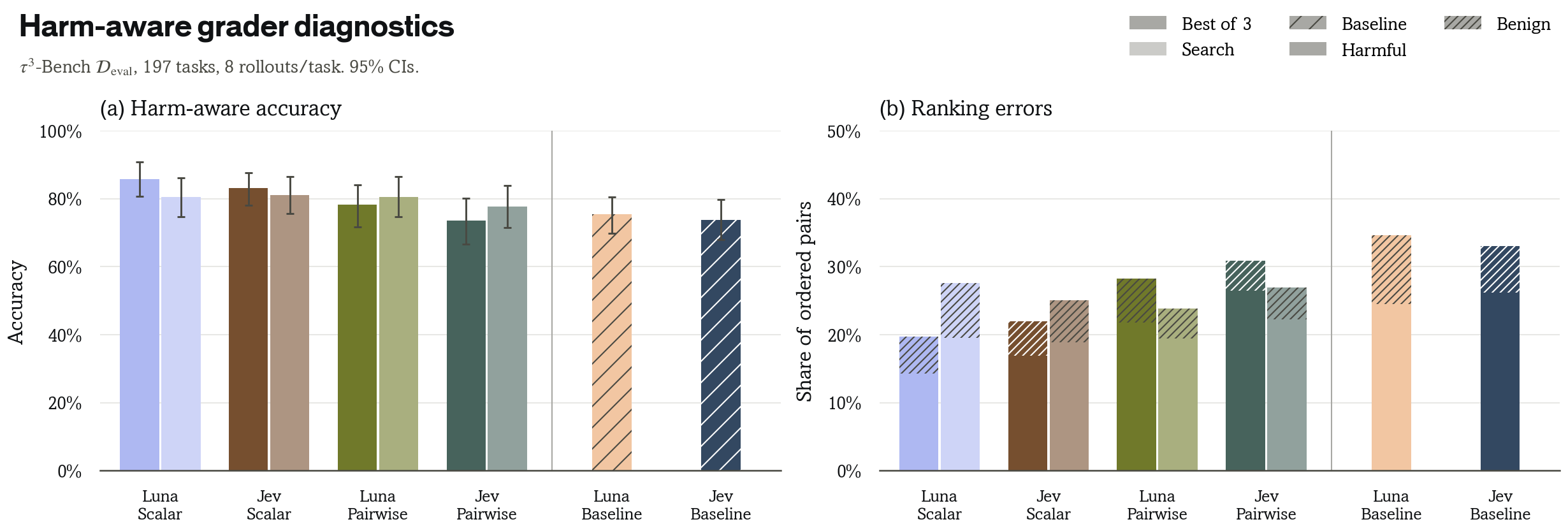
Harm-aware ranking accuracy focuses on grading errors that could change the direction of a training update [Shang et al., 2026]. For example, if a response already scores below the group average, then giving it an even lower score still pushes the policy away from that response, and so it is not as meaningful of a mistake. But an error that causes us to reinforce a bad response, or discourage a good one, is more consequential.
Within-task Spearman correlation measures agreement across the full ranking of responses to each task:
Here, are the sampled responses to task , and is Spearman rank correlation. Unlike pairwise accuracy, this metric also measures how far apart two rankings are. In this case, moving a response from first to last in ranking matters more than swapping two adjacent responses.
These measurements let us compare grader candidates without needing to train a policy for each one. They tell us how well the metagrader agrees with the expert criteria on the starting policy, although the training experiments are still needed to see whether that agreement translates into better models.
Scalar versus rubric graders
What scalar graders miss
The difference between scalar and rubric grading is particularly noticeable on Harvey-LAB. In Figure 10, we compare eight attempts at the same legal task under the expert grader, the scalar metagrader, and the rubric metagrader.
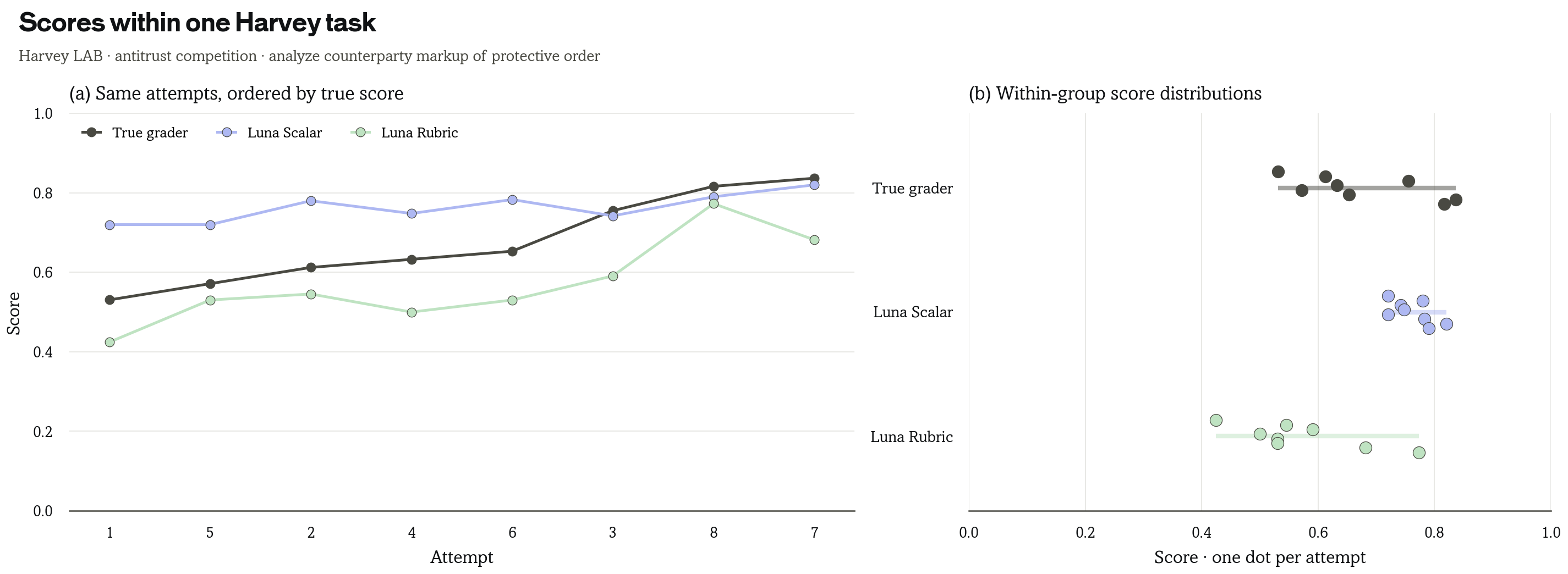
The scalar grader assigns similar scores to responses that the expert grader separates. These memos often differ on fairly specific requirements, which can get lost if the judge is asked for a blanket assessment of the entire response.
Rubric grading handles this somewhat better by checking individual criteria. On -Bench, where outcomes are binary successes or failures, the scalar approach was sufficient. This suggests that the choice of grading format should depend partly on what are the kinds of errors we want the grader to tell apart.
Are the generated rubrics any good?
High levels of agreement with the expert grader still doesn't fully tell us if the generated rubric contains the right requirements or not. A rubric could rank responses correctly while relying on its own generated criteria that happen to be vague, unsupported, or missing important details.
So, we decided to dig deeper and analyze the generated criteria themselves. We analyzed the expert and generated rubrics for 250 Harvey-LAB evaluation tasks where both were available, and had an auditor (GPT-6-Astra) look at the task and its source documents, but not which system wrote each criterion. We followed the rubric definitions from prior work [Shao et al., 2025] and checked three properties:
- Specificity: Whether a criterion is asking for a concrete fact, conclusion, or calculation, rather than a general topic or quality.
- Grounding: Whether the requirement is supported by the source documents, contradicted by them, or cannot be verified from the available information.
- Omission: Whether a response could leave out the content the criterion is meant to check and still pass it.
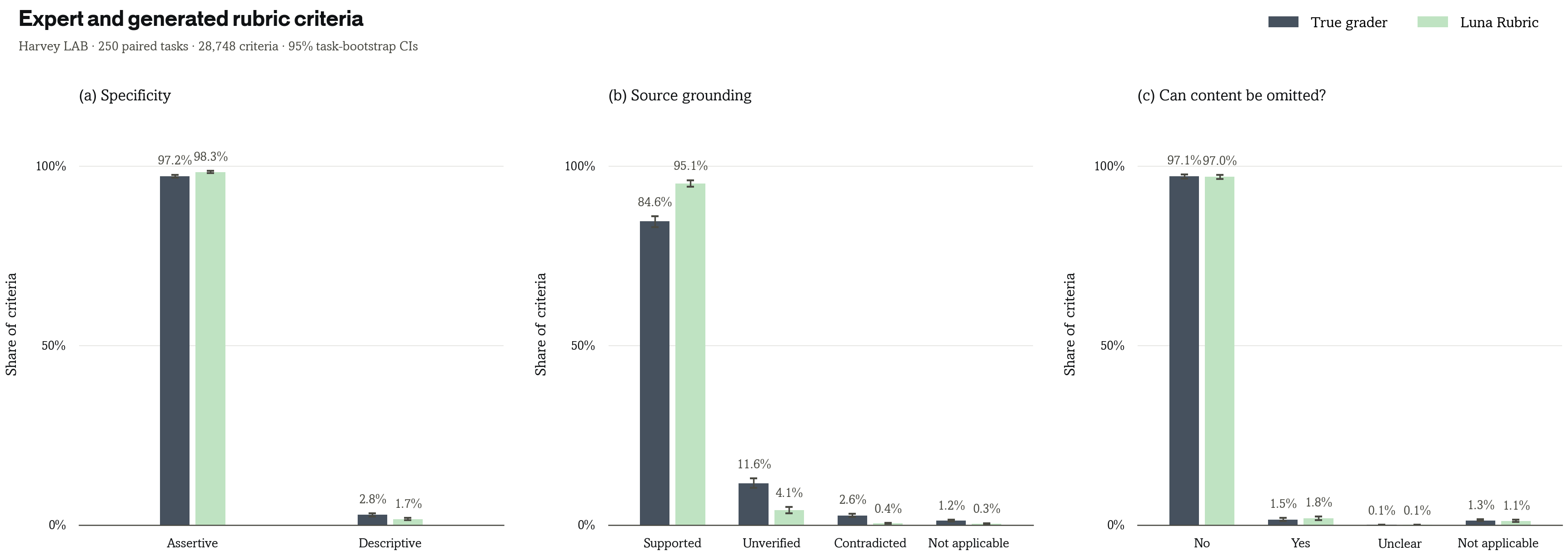
The generated rubrics had a higher proportion of criteria supported by the source documents: 95% compared with 85% for the expert rubrics. This difference was also fairly consistent, with generated rubrics having a higher supported fraction on 211 of the 250 tasks.
Some expert criteria were so far as directly contradicted by the documents. For example, one specified a dollar amount that didn't actually follow from the share count, and another one claimed that a policy lacked role definitions that were actually present in the text.
There are important caveats. The auditor itself was a model (Luna), which also generated the rubrics, so the evaluation isn't independent. We also instructed the auditor to use only the provided sources, without any access to additional information. An expert criterion marked as unverified might need to rely on legitimate domain knowledge that wasn't in those documents.
We saw another difference in an earlier Nemotron training experiment (Appendix A). Models trained with generated and expert rubrics achieved similar all-pass rates, but the generated-rubric model satisfied 60% of individual expert criteria, compared with 67% for the expert-rubric model.
The two rubric sets don't always test exactly the same requirements. Generated rubrics tend to contain a somewhat larger set of criteria, and sometimes check a requirement more explicitly than the expert version.
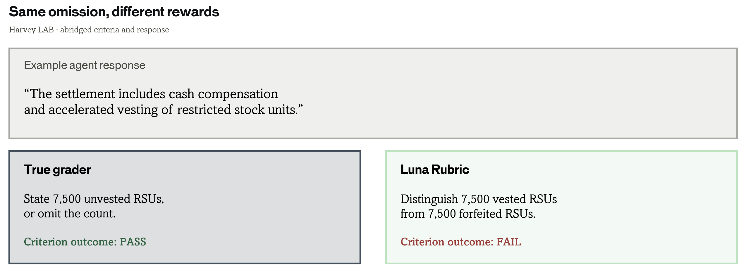
For example, Figure 12 shows a case where a response could omit an RSU count and still pass the expert criterion, while the generated criterion requires the count explicitly.
So the rubric audit gives us some reason to believe that generated criteria can be more specific and better grounded in the available documents. But these differences also mean that training on generated rubrics won't necessarily optimize exactly the same requirements that were defined in the expert rubrics.
Limits of the search
One limitation we found is that evolutionary search can overfit to the examples that were used to select a metagrader.
As we search over more candidates, it’s possible that we can improve the agreement on the selection set without necessarily improving on held-out tasks. We observed this behavior in our experiments with evolutionary metagrader search (Appendix D).
This matters because the number of expert-labeled examples is deliberately small. A search method can unintentionally learn the nuances of the seed set of examples rather than learn the general rules for grading new tasks.
For now, our experiments use separate construction, selection, and evaluation sets, and we validate the selected graders through downstream training. Better ways to control overfitting during search (ie inject regularization), and to choose which new examples experts should label, remain open questions.
Where this goes
On -Bench, a metagrader built from 60 labeled tasks recovers most of the gain from training on the true grader, in distribution and on an unseen domain. On Harvey-LAB, a policy trained on generated rubrics matches one trained on the expert rubrics, from 48 labeled construction tasks and 48 labeled selection tasks.
Continual Grading handles one half of continual learning, deciding what the model should be rewarded for. Our companion post, You Only Rollout Once, handles the other half, learning from production traffic without rebuilding it in a simulator. Together, both of these insights allow you to train a model on the work it does every day, against a reward a trusted set of experts have defined.
Production traffic drifts, so a grader written once goes stale. Because a metagrader is a prompt and harness, it can be cheaply re-optimized on expert labels for the policy's latest rollouts, keeping pace with the policy and the task mix. Search that doesn't overfit [Xu et al., 2026], and choosing which rollouts experts label next, would make each refresh cheaper.
Trajectory
Continual Grading is available as a research preview in Trajectory. Experts label a few examples, Trajectory searches for a metagrader, and its grades go straight into training.
If you're interested in this research, join us.
Citation
Please cite this work as:
Kale, Neil; Trajectory Labs. “Continual Grading.” Trajectory Labs: Field Notes, November 2026. https://trajectory.ai/field-notes/continual-gradingOr use the BibTeX citation:
@misc{trajectory2026continualgrading,
  author       = {Kale, Neil and Trajectory Labs},
  title        = {Continual Grading},
  howpublished = {Trajectory Labs: Field Notes},
  month        = {November},
  year         = {2026},
  url          = {https://trajectory.ai/field-notes/continual-grading},
}
References
- Agrawal, L. A., et al. (2025). GEPA: Reflective Prompt Evolution Can Outperform Reinforcement Learning. arXiv:2507.19457.
- Barres, V., et al. (2025). -Bench: Evaluating Conversational Agents in a Dual-Control Environment. arXiv:2506.07982.
- Bradley, R. A., and Terry, M. E. (1952). Rank Analysis of Incomplete Block Designs: I. The Method of Paired Comparisons. Biometrika 39, 324–345. doi:10.2307/2334029.
- Findeis, A., et al. (2024). Inverse Constitutional AI: Compressing Preferences into Principles. arXiv:2406.06560.
- Gao, L., Schulman, J., and Hilton, J. (2022). Scaling Laws for Reward Model Overoptimization. arXiv:2210.10760.
- Grupen, N., Pereyra, G., and Pereyra, J. (2026). Open-Sourcing Harvey's Long Horizon Legal Agent Benchmark. Harvey. Blog post.
- Gunjal, A., et al. (2025). Rubrics as Rewards: Reinforcement Learning Beyond Verifiable Domains. arXiv:2507.17746.
- Lambert, N. (2025). Reinforcement Learning from Human Feedback, Chapter 5: Reward Models. rlhfbook.com.
- Lambert, N., et al. (2024). RewardBench: Evaluating Reward Models for Language Modeling. arXiv:2403.13787.
- Lee, Y., Nair, R., Zhang, Q., Lee, K., Khattab, O., and Finn, C. (2026). Meta-Harness: End-to-End Optimization of Model Harnesses. arXiv:2603.28052.
- Shang, S., Strauss, H., Wei, S., Arora, S., and Razin, N. (2026). When Errors Can Be Beneficial: A Categorization of Imperfect Rewards for Policy Gradient. arXiv:2604.25872.
- Shao, R., et al. (2025). DR Tulu: Reinforcement Learning with Evolving Rubrics for Deep Research. arXiv:2511.19399.
- Shao, Z., et al. (2024). DeepSeekMath: Pushing the Limits of Mathematical Reasoning in Open Language Models. arXiv:2402.03300.
- Tan, S., et al. (2024). JudgeBench: A Benchmark for Evaluating LLM-based Judges. ICLR 2025. arXiv:2410.12784.
- Xu, R., Chen, Y., et al. (2026). Harness²: Recursive Agent Harnessing for an Open World. arXiv:2610.14224.
- Yao, S., et al. (2024). -bench: A Benchmark for Tool-Agent-User Interaction in Real-World Domains. arXiv:2406.12045.
- Zhang, A. (2026). Harnesses. Blog post.
- Zheng, C., et al. (2025). Group Sequence Policy Optimization. arXiv:2507.18071.
- Zheng, L., et al. (2023). Judging LLM-as-a-Judge with MT-Bench and Chatbot Arena. arXiv:2306.05685.
- Zhou, H., Ye, K., Xu, E., Zhu, J., Yang, Y., Gong, S., and Shi, C. (2026). Demystifying Group Relative Policy Optimization: Its Policy Gradient is a U-Statistic. arXiv:2603.01162.
Appendix
A. Data splits
-Bench
We use 375 tasks: the standard Tau2 base sets for airline (50), retail (114) and telecom (114), plus all 97 banking tasks from Tau3, all held out for eval. We adopt the standard Tau2 train-eval split (178/100). The tasks in have true graders, but we hide them to simulate unlabeled production tasks. The true grader checks database state and required communications. We also train on and , which doesn't leak and keeps data parity with public -Bench results.
| Domain | Metagrader seed, | Metagrader selection, | Train, | Eval, |
|---|---|---|---|---|
| Labeled | Labeled | Unlabeled | Labeled | |
| Airline | 5 | 5 | 20 | 20 |
| Retail | 12 | 13 | 49 | 40 |
| Telecom | 13 | 12 | 49 | 40 |
| Banking | — | — | — | 97 |
| Total | 30 | 30 | 118 | 197 |
Harvey-LAB
There is no standard train-eval split, so we hold out three domains (Immigration, Tax, Trusts; 138 tasks) and follow the Artificial Analysis evaluation protocol for the other 24 domains (five eval tasks each, 120 total). The remaining 1,752 tasks are split into domain-stratified seed, selection and training sets.
| Domain | Metagrader seed, | Metagrader selection, | Train, | Eval, |
|---|---|---|---|---|
| Labeled | Labeled | Unlabeled | Labeled | |
| 24 other domains | 2 each | 2 each | —— | 5 each |
| Immigration | 0 | 0 | 0 | 27 |
| Tax | 0 | 0 | 0 | 34 |
| Trusts, estates & private client | 0 | 0 | 0 | 77 |
| Total | 48 | 48 | 1,656 | 258 |
Current Harvey training comparison
Figures 8–9 use Qwen3.6-35B-A3B (35B total / 3B active), three seeds each for true expert-rubric and frozen Luna-rubric rewards. Both train on partial criterion rewards over the same 1,656 tasks. The 258-task evaluation split contains 120 ID and 138 OOD tasks, with one attempt per task every five updates; reported evaluation is native expert-rubric all-pass.
The shared setup is GSPO, 8 tasks × 8 attempts before filtering, LoRA rank 32, constant learning rate , temperature 1, top-p 1, top-k −1, a fixed 131,072-token total output cap, and 65,536 tokens per turn. Training and evaluation concurrency are 192 and 128. All six seeds completed 150 updates. Continuations toward 20,000 consumed training rollouts each are running; Figure 8 shows training through 15,000 rollouts; Figure 9 averages evaluations at 12,500–17,500 rollouts.
Figure 9 averages settled evaluations within 12,500–17,500 consumed training rollouts, first within each seed and then equally across the three seeds per arm. True-grader seeds contribute 11 / 13 / 10 checkpoints; Luna-rubric seeds contribute 12 / 12 / 13. The shared base pools all six step-zero evaluations. Failed attempts count as zero; pending and cancelled evaluations are excluded. The task bootstrap uses 10,000 draws with seed 0, resampling matching tasks jointly across conditions while preserving the 120-ID / 138-OOD composition. These intervals are conditional on the fixed seeds and checkpoints.
Earlier Harvey training comparison
For historical reference, the earlier Nemotron comparison used the original 1,890 training / 120 evaluation split. Figures 8–9 now use the Qwen runs on the 258-task split. The historical policy is Nemotron 3.5 Super (120B total / 12B active), trained with GSPO, LoRA rank 32 and learning rate . Evaluation uses one attempt per task every five updates. The synthetic run uses the earlier Luna rubric metagrader, RL3, whose task rubrics were generated before policy training.
| Policy / checkpoint | Expert-rubric all-pass | Expert criteria met |
|---|---|---|
| Base | 5/120 (4.2%) | 76.7% |
| Expert-rubric training, step 55 | 17/120 (14.2%) | 66.9% |
| Synthetic-rubric training, step 25 | 19/120 (15.8%) | 60.0% |
All three rows cover 120 tasks, including the saved replacements for infrastructure failures. Token-limit failures score zero in both metrics. The checkpoints were selected separately for all-pass, and the improvement in all-pass does not imply more expert criteria met.
This is an earlier feasibility comparison. There is one run per condition, training settings changed across continuations, and five evaluation tasks overlapped with the grader-builder's labeled examples. It is not a controlled grader-only ablation or a result for the newly built metagraders.
- Expert-rubric lineage: 1062992 (0–26) → 1063357 (27) → 1063439 (28–42) → 1063598 (43–49) → 1063645 (50–100) → 1064749 (101–200).
- Synthetic-rubric lineage: 1063619 (0–22) → 1063687 (23–90) → 1064755 (91–116).
- Displayed checkpoints: expert 1063645/55; synthetic 1063687/25, with three failed eval tasks completed by backfill 1064865; base 1063586 + 1063612.
B. Models
The metagrader uses sandboxed GPT-6-Luna (openai/gpt-6-luna) and/or Jev (typesafe/jev-1.14) as judge models. The meta-harness uses GPT-6-Astra (openai/gpt-6-astra(reasoning_effort="max")); its sandbox disables web search, restricts mounts, rejects hosted tools and disables remote-file retrieval. Offline -Bench traces come from Nemotron 3.5 Lightning (nvidia/NVIDIA-Nemotron-3.5-Lightning-30B-A3B-BF16), and offline Harvey-LAB traces come from Nemotron 3.5 Super (nvidia/NVIDIA-Nemotron-3.5-Super-VL-120B-A12B-BF16). The current Harvey training comparison uses Qwen3.6-35B-A3B (Qwen/Qwen3.6-35B-A3B, 35B total / 3B active).
-Bench training runs use GSPO with about 40k rollouts per run, learning rate 1e-4, 64k context, and a length penalty. The penalty applies to the training reward only. Held-out evaluation uses the true grader without it, and the baseline-judge arm shares the same penalty. Training curves are plotted against training rollouts, so runs with different batch sizes line up. Evaluation is one rollout per task every 5 updates, so the eval curves are noisier than training reward. Figure 6 and the reported training gains average evaluations at 35,000–45,000 rollouts, first within each seed and then equally across the three seeds per arm. The shared base pools all nine step-zero evaluations.
C. Metric details
Tau candidate selection and search used the original metric: scalar comparisons used a 0.1 tolerance and half credit for predicted ties, and pairwise comparisons used symmetrized direct decisions with half credit for ties. All reported ranking-accuracy figures use exact scalar ordering and pairwise wins-only aggregate reward ranking, with zero credit for predicted ties. The search curve recomputes this metric for the actual selected grader at each round, using saved scores. Candidate selection and search were not rerun.
After ignoring benign errors, the selected Luna scalar metagrader rises from 80.3% to 85.7% ranking accuracy on .
D. Evolutionary search on -Bench
Following Meta-Harness [Lee et al., 2026], we also ran a 20-iteration evolutionary search. At each iteration, the proposer reads every prior candidate's code, traces and results on and proposes three new metagraders. In all four settings, search climbs ranking accuracy on .
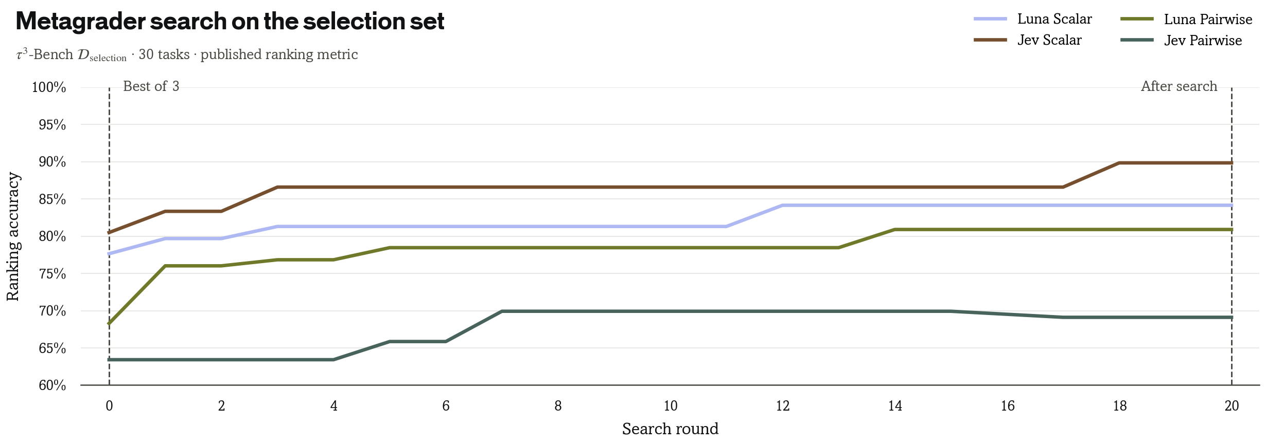
On held-out , the gains don't hold. Confidence intervals overlap, and search lowers accuracy for both scalar graders (Luna 80.3% → 72.4%, Jev 78.0% → 74.9%) while raising it for both pairwise graders (Luna 71.8% → 76.2%, Jev 69.1% → 73.1%).
E. Meta-harness prompts
The baseline synthetic grader prompt is:
Grade this trace from 0 to 1, where 0 means failure and 1 means full success.The default meta-harness prompt is:
Build a reusable program for Luna to grade completed outputs during RL training, so that better and worse attempts on the same task receive scores aligned with the task’s true grader. Some tasks are provided with their true graders and prior criterion-level grades; prior attempts vary in quality and are not gold-standard answers, and new tasks’ true graders will be unavailable.To enforce pairwise grading:
Build a reusable program for Luna to compare two attempts at the same previously unseen task, aiming to identify which attempt would receive the higher score under the true grader and allowing ties. Some tasks are provided with their true graders and prior criterion-level grades; prior attempts vary in quality and are not gold-standard answers, and new tasks’ true graders will be unavailable.To enforce rubrics:
Build a reusable program that writes rubrics from task descriptions and source documents for Luna to grade completed outputs during RL training, so that better and worse attempts on the same task receive scores aligned with the task’s true rubric. Some tasks are provided with their true graders and prior criterion-level grades; prior attempts vary in quality and are not gold-standard answers, and new tasks’ true graders will be unavailable.To enforce pairwise grading with rubrics:
Build a reusable program that writes rubrics from task descriptions and source documents for Luna to compare two attempts at the same previously unseen task, aiming to identify which attempt would receive the higher score under the true grader and allowing ties. Some tasks are provided with their true graders and prior criterion-level grades; prior attempts vary in quality and are not gold-standard answers, and new tasks’ true graders will be unavailable.When using Jev as a grader, we replace references to Luna with Jev and append:
You will use Jev, a calibrated decision model, as the judge model. Documentation on Jev is available in /docs/jev.F. Rubric criteria audit
Blind audit of every criterion in the expert and generated rubrics on the 250 Harvey-LAB eval tasks where both exist. The auditor is Luna, shown the task and its sources but not the criterion's author. Shares are task means with bootstrap 95% confidence intervals.
| Share of criteria, task mean (95% CI) | Expert | Generated |
|---|---|---|
| Criteria per task | 54.9 | 60.1 |
| Assertive | 97.2% [96.7, 97.6] | 98.3% [98.0, 98.6] |
| Supported by sources | 84.6% [83.0, 86.0] | 95.1% [94.2, 96.0] |
| Unverified | 11.6% [10.3, 13.0] | 4.1% [3.2, 5.0] |
| Contradicted | 2.6% [2.2, 3.1] | 0.4% [0.3, 0.6] |
| Omission forbidden | 97.1% | 97.0% |