Choosing the Trainable Geometry for Agentic RL

At Trajectory, we’re building the infrastructure for enterprises to train agents that continually learn as users interact with them. As open-source models cross the trillion-parameter mark, we need ways to teach them new skills efficiently without harming their pretrained knowledge (catastrophic forgetting) or their ability to continually learn (model plasticity).

Prior work attacks this problem from several different angles. Gradient-free algorithms for prompt optimization and harness engineering enable new skills without making any update to the model weights, for example, by adding search tools or in-context examples to augment the model with relevant knowledge. In this post, we focus on parameter-efficient finetuning (PEFT) algorithms, which update a subset of model weights and intelligently choose a subspace to update over.

We start from the most common PEFT algorithm: Low-Rank Adaptation (LoRA) [1]. To understand LoRA, recall that transformer models consist of layered blocks, each roughly made up of an attention module, MLP module, and some regularizations.

During pretraining, model gradient updates typically propagate through all the weights. Full finetuning (FFT) does the same full update in post-training, which teaches the model specific downstream tasks. However, FFT is slow and expensive, particularly for large models, and runs the risk of catastrophic forgetting: overfitting the model to the selected task and losing general capabilities (see Figure 1).

Full fine-tuning and LoRA responses to math and chat prompts — Figure 1. When full finetuned for math reasoning, the base model begins outputting math formatting in response to ordinary chat questions as well. When trained with LoRA, the model still learns the math problem, but does not lose its chat behavior.

To combat these problems, LoRA freezes each pretrained weight matrix $W_0$ and trains two much smaller rank- $r$ matrices, $A$ and $B$ . The finetuned weight matrices are set as $W = W_0 + AB$ . This cuts the number of trainable parameters and the optimizer memory needed for downstream training.

LoRA math

To understand this blog post, we'll need a small toolkit of basic linear algebra. Feel free to skip ahead if you’re already familiar with matrix factorization!

A matrix is a linear map. It transforms an input vector $x$ into an output $y = Wx$ . The rank of $W$ is the number of independent directions that its outputs can span. Given a matrix $W \in \mathbb{R}^{m \times n}$ , we say $W$ has rank $r$ if it can be written as a product,

W=AB

where $A ∈ \mathbb{R}^{m×r}$ , $B ∈ \mathbb{R}^{r×n}$ . Note that the product $AB$ uses $rm + rn$ parameters instead of $mn$ , so this compresses the matrix. If $r \ll \min{(m,n)}$ , we call $W$ a low-rank matrix and $AB$ a low-rank factorization.

For a $4096 \times 4096$ weight matrix with rank $r = 32$ , the low-rank factorization would have $32 × (4096 + 4096) ≈ 262\text{k}$ trainable parameters instead of $16.8\text{M}$ .

Note, in general, weight matrices $W$ can’t be written as $AB$ . The initial model weights tend to be near full-rank, and can’t be compressed losslessly.

Instead, a low-rank adapter takes an existing weight matrix $W$ and writes it as $W = W_0 + AB$ . For standard LoRA, we initialize with $W_0 = W$ , $A \sim \mathcal{N}(0, \sigma^2)$ (random matrix), and $B = \mathbf{0}$ . The adapter $AB$ therefore starts at zero, and the initialization is equivalent to full finetuning since $W = W_0 + A \cdot \mathbf{0}$ .

Since the update passes through an $r$ -dimensional bottleneck, LoRA constrains how the model can change. The factors rotate during training, so the weight matrices don’t stay inside a fixed subspace. However, at any point, the difference between the base weights $W_0$ and the finetuned weights $W_0 + AB$ must be compressible into rank $r$ .

To visualize this in 3D, we let $W \in \mathbb{R}^{2 \times 2}$ with low-rank adapters $A,B$ at $r=1$ . If we fix the top-left entry of $AB$ , the remaining entries are constrained as shown below. In higher-dimensions, we can’t visualize this constraint as easily, but it still exists: $W_0 + AB$ does not cover all possible $m \times n$ matrices.

Despite the representation constraint, these low-rank updates are surprisingly effective. Prior work from Schulman et al. [2] finds that for reinforcement learning, rank-1 adapters are often as effective as full finetuning.

In 2D, a rank-1 adapter is only 1-dimension smaller than the entire space. However, the attention weight matrices for a large language model are much higher-dimensional. For example, a $Q$ projection for Qwen3-4B can map 2560 → 4096. In a $2560 \times 4096$ weight matrix, a rank-1 adapter occupies a small fraction of the representation space and has very low coverage.

The fact that rank-1 LoRA works suggests that models are not capacity-constrained in learning new tasks. Biderman et al. [3] find that LoRA also forgets less than full finetuning, substantiating the theory that low-rank updates are less likely to overwrite pretrained skills.

Another way to initialize: PiSSA

One issue with vanilla LoRA is that it throws away a free prior. Since $A$ is random and $B$ is zero, the updates begin on a random subspace. Instead, suppose that the directions the model stretched most during pre-training are the directions that matter for post-training too. Base models are often midtrained well on tasks we care about downstream such as coding, law, and biology [12]. If we could compute the $r$ “most important” dimensions of each weight matrix, it could make sense to initialize LoRA along these dimensions.

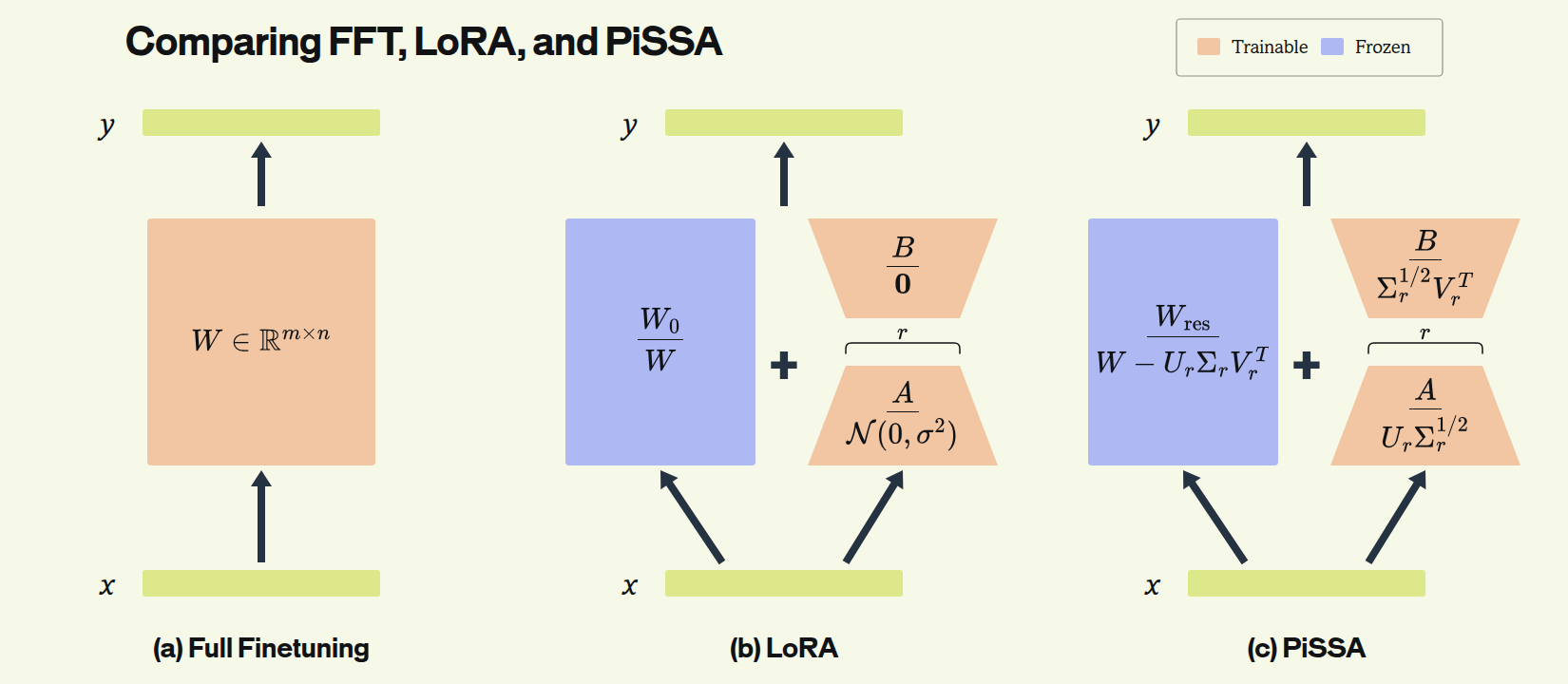
Full fine-tuning, LoRA, and PiSSA initialization — Figure 2. Comparing initializations for FFT, LoRA, and PiSSA.

PiSSA [4] starts exactly there. It computes the singular value decomposition (SVD) of each weight matrix $W$ which produces two matrices $U$ and $V$ such that the scaled first $r$ columns of $U$ , $U_r$ , and the scaled first $r$ rows of $V^\top$ , $V_r$ , are exactly the $A$ and $B$ such that $AB$ is the closest possible rank- $r$ approximation of $W$ .

SVD image reconstructions at increasing ranks — Figure 3. Comparing SVDs of matrices across various k. Source: NASA, original image.

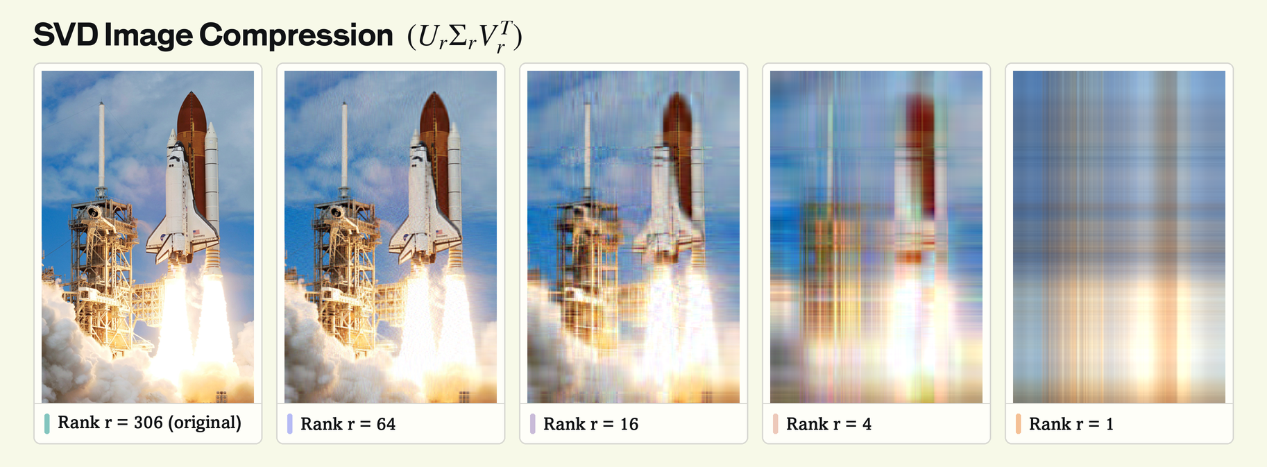
Here, closest means $U_rV_r^\top$ minimizes the Frobenius norm, $\min_{AB}{\|W - AB\|_F}$ .

To ensure equivalence, PiSSA then sets the frozen weights $W_0$ to the residual matrix $W_{res} = W - AB.$ The residual $W_{res}$ and adapter $AB$ still add up to the original $W$ at step 0.

PiSSA therefore starts as the same pretrained model and uses the same low-rank adapter architecture as LoRA. The only difference is the initialization of the trainable and frozen weights, and thus which low-rank manifold the weights are fixed to.

SVD and PiSSA math

The singular value decomposition (SVD) writes a matrix as

W = U\Sigma V^\top.

The columns of $V$ are orthonormal input directions, the columns of $U$ are the corresponding orthonormal output directions. The singular values in $\Sigma$ say how strongly the matrix acts along each pair of directions. They are ordered from largest to smallest, so the first $r$ ranks are the strongest ones.

A 2×2 example.

W_0 = \begin{bmatrix} 3 & 1 \\ 1 & 3 \end{bmatrix} = \frac{1}{\sqrt{2}}\begin{bmatrix} 1 & 1 \\ 1 & -1 \end{bmatrix} \begin{bmatrix} 4 & 0 \\ 0 & 2 \end{bmatrix} \frac{1}{\sqrt{2}}\begin{bmatrix} 1 & 1 \\ 1 & -1 \end{bmatrix} = U\,\Sigma\,V^\top.

The singular values are 4 and 2, and the singular directions mix the coordinates rather than lying on them. At rank 1, the principal component and residual are

A_0B_0 = \begin{bmatrix} 2 & 2 \\ 2 & 2 \end{bmatrix}, \qquad W_{res} = W_0 - A_0B_0 = \begin{bmatrix} 1 & -1 \\ -1 & 1 \end{bmatrix}.

Their sum is still the original $W_0$ , and the trainable factors are just $A_0 = \sqrt{2}\,(1,1)^\top$ and $B_0 = \sqrt{2}\,(1,1)$ .

Initializing PiSSA.

The SVD has several nice properties. For one, it lets us find $A,B$ of rank $r$ such that $AB$ solves $\min_{AB}{\|W - AB\|_F}$ .

We do this by defining the top-r component of matrix $W$ as

W_r = U_{[:,:r]}\Sigma_{[:r,:r]}V_{[:,:r]}^\top=U_r\Sigma_rV_r^\top.

PiSSA factors this component as

A = U_r\Sigma_r^{1/2}, \qquad B = \Sigma_r^{1/2}V_r^\top,

and defines

W_{res} = W - AB.

This initialization starts the optimizer in the directions where the pretrained weights already act most strongly, and freeze the remaining directions into $W_{res}$ .

Interactive demo

To understand why PiSSA helps downstream training, let’s consider a simplified example. In the demo below, we start with weight matrix $W \in \mathbb{R}^{3 \times 3}$ . Note that every $3 \times 3$ matrix forms a triangle in 3D, so we can represent the weight matrix as a periwinkle triangle. We also set a target matrix shown by a teal triangle.

We set $W = W_0 + AB$ , where $W_0$ is the frozen weights (dashed navy) and $A$ and $B$ are both rank-1 matrices (vectors). By selecting LoRA or PiSSA , you can change the initialization from $W_0 = W,\; A \sim \text{random},\; B = \mathbf{0}$ to $W_0 = W_{res},\; A =U_r,\; B = V_r$ . Note that choosing LoRA or PiSSA doesn’t change the initial $W$ in periwinkle.

Press Train to simulate gradient descent along the Frobenius norm between the two matrices.

In standard LoRA, B starts at zero, so A receives zero gradient on the first step. B can update, but that update is projected through the random initial A. Because of this, the matrix starts by moving in an arbitrary direction and takes a while to converge. PiSSA starts with both factors nonzero and aligned with the principal singular directions, so both factors receive structured gradients immediately.

Moreover, these gradients are aligned with the teal target triangle, which represents an aligned task where the important learning directions are similar to the strongest directions in the original weights. A real world example of this is taking a model that has been trained to solve agentic retail and airline tasks, and teaching it to use insurance software. In theory, the model needs similar patterns of tool use and reasoning, so the pretrained directions are aligned with the post-training task.

To the contrary, suppose we have a model like Qwen-3-Coder that is already specialized for coding. The PiSSA initialization may mostly contain directions relevant for coding, so if we try to train this model to redline legal documents, it may fail. Select the Orthogonal task option to simulate this setting, where PiSSA stalls out because its representational manifold does not include the orthogonal target, whereas LoRA succeeds albeit slowly.

Evaluating PiSSA for Reinforcement Learning

Work from our friends at Thinking Machines has shown how effective LoRA can be for reinforcement learning. There is a broad "low-regret" regime where even rank-1 adapters are empirically close to full fine-tuning [2]. While the original PiSSA work showed the algorithm was effective for supervised finetuning, it remains unclear whether PiSSA would work for reinforcement learning. RL is often less stable, since each update changes the policy that generates the next round of training data. Since PiSSA makes early updates larger, it could enable faster progress toward useful behavior, or faster drift away from policies that were producing good data.

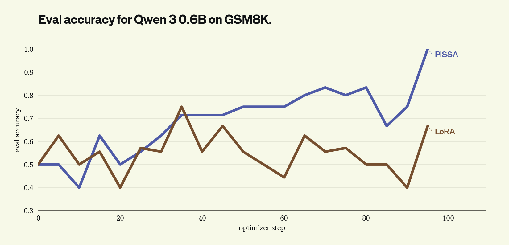
To test whether PiSSA initialization improves RL training on real tasks, we ran RL training jobs for Qwen 3 0.6B on GSM8K, Qwen 3 4B on Tau Bench, and Qwen 3.6 27B on SuperGPQA. The LoRA and PiSSA jobs both applied rank-32 adapters on the attention and MLP projections. Further infrastructure details are included in Contributions to SkyRL [PR Link] below. With SkyRL, we also provide example scripts to easily reproduce our Qwen 3 0.6B experiments.

We note that concurrent work found that for RL, PiSSA was less stable than LoRA at fixed learning rate [5], and the original PiSSA work found that for SFT the optimal learning rate for PiSSA tends to be smaller than for LoRA [1, Appendix L]. Since PiSSA begins with both adapters non-zero and acts on the most active directions in the weight space, it also makes intuitive sense that PiSSA would need lower learning rate. In our experiments, we fix the PiSSA learning rate at 2e-5 and the LoRA learning rate at 1e-4 for Qwen3-27B on SuperGPQA. We find that PiSSA is unstable at 1e-4, and LoRA does not climb at all at 2e-5 for this task. For Qwen3-4B on Tau, we use 1e-4 for both PiSSA and LoRA. For Qwen3-0.6B, we use 3e-6 for both PiSSA and LoRA, so we can do a fair LoRA/PiSSA comparison based on the Frobenius distance between the base and learned weights and the KL divergence between the base and target policy.

Experimental Results

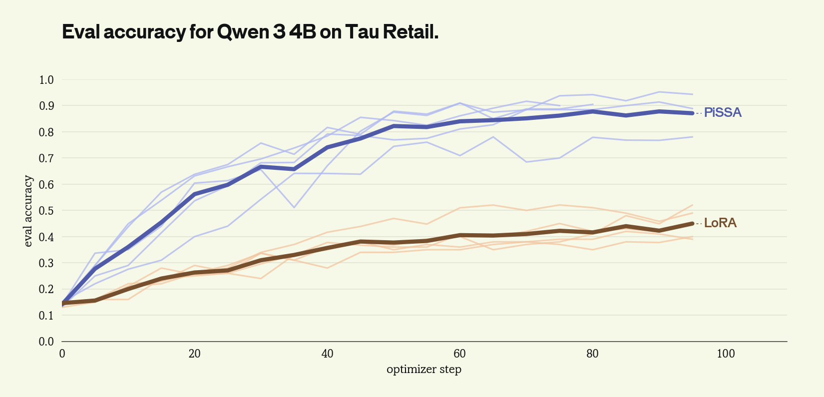
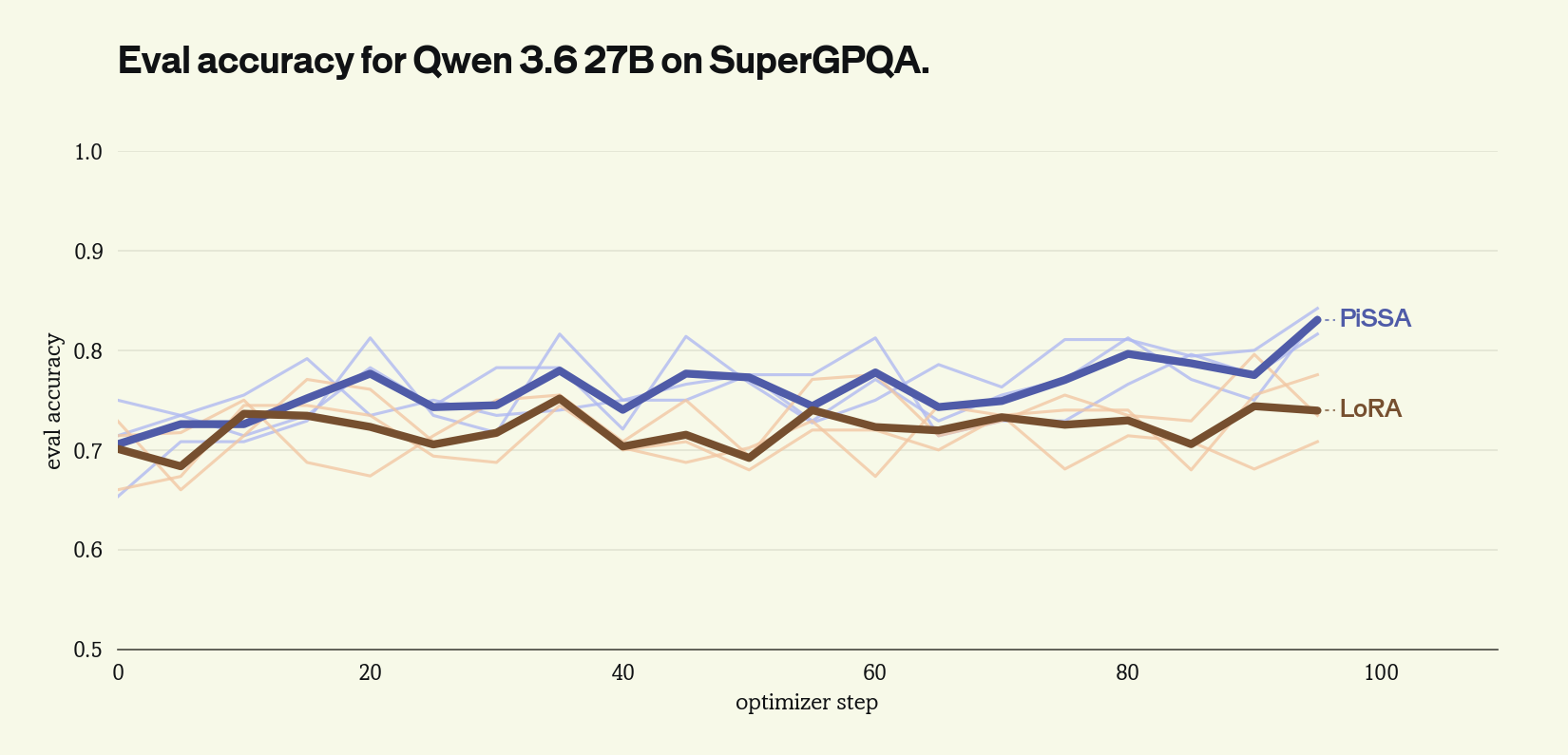
We find that across all three model-task pairs, PiSSA outperforms LoRA with statistical significance.

Eval accuracy against optimizer step, for Qwen 3 4B on Tau Retail, Qwen 3.6 27B on SuperGPQA, and Qwen 3 0.6B on GSM8K. Thin lines are individual runs, and the thick line is their mean. The 4B panel has five runs per arm, the 27B panel has three, and the 0.6B panel has one.

Qwen3 4B evaluation accuracy on Tau Retail — Figure 4. Eval accuracy for Qwen 3 4B on Tau Retail.

Qwen3.6 27B evaluation accuracy on SuperGPQA — Figure 5. Eval accuracy for Qwen 3.6 27B on SuperGPQA.

Qwen3 0.6B evaluation accuracy on GSM8K — Figure 6. Eval accuracy for Qwen 3 0.6B on GSM8K.

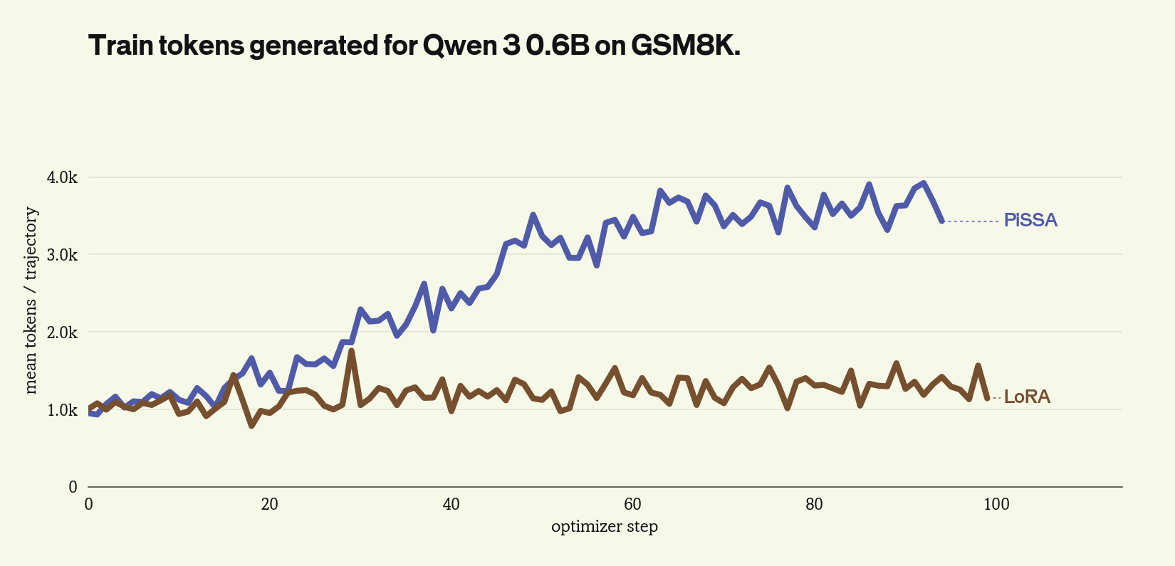
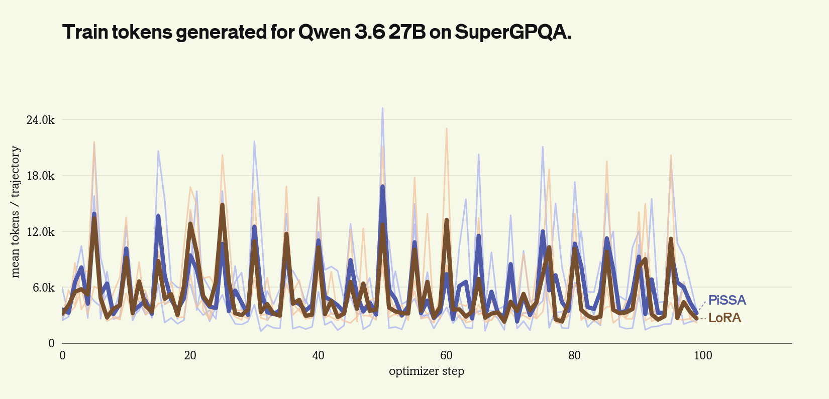
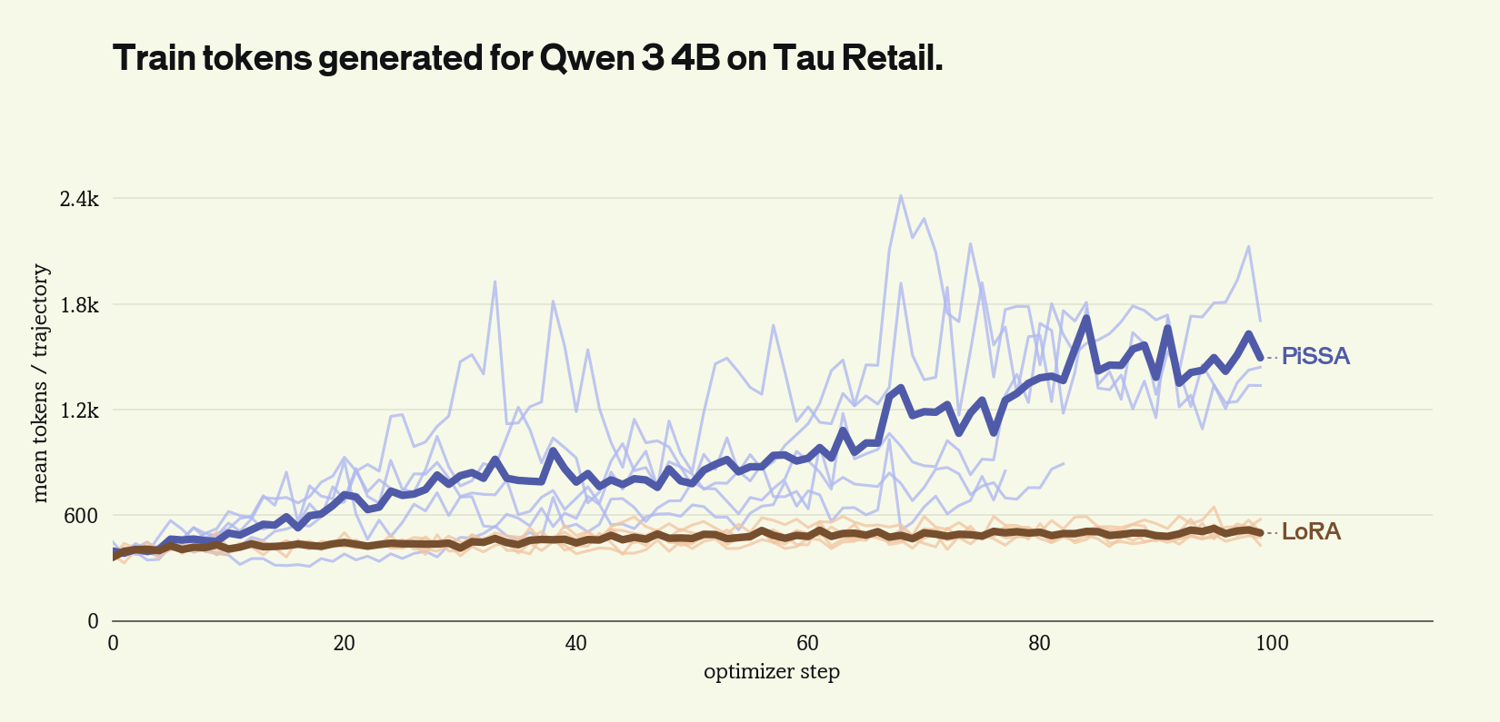
On Tau and GSM8K, which involve multiple steps of tool-calling, the PiSSA policies grow significantly more verbose than the LoRA policies. On SuperGPQA, a single step task, the two initializations produce similarly verbose policies.

Mean tokens generated per trajectory during training, for the same runs as Figures 4–6, in the order Qwen 3 0.6B on GSM8K, Qwen 3.6 27B on SuperGPQA, and Qwen 3 4B on Tau Retail. On the 0.6B and 4B runs, the PiSSA policies grow about three times longer than the LoRA policies over 100 steps. On the 27B runs the two arms stay together, so the accuracy gain at that scale arrives without longer outputs.

Qwen3 0.6B mean training tokens per trajectory on GSM8K — Figure 7. Train tokens generated for Qwen 3 0.6B on GSM8K.

Qwen3.6 27B mean training tokens per trajectory on SuperGPQA — Figure 8. Train tokens generated for Qwen 3.6 27B on SuperGPQA.

Qwen3 4B mean training tokens per trajectory on Tau Retail — Figure 9. Train tokens generated for Qwen 3 4B on Tau Retail.

Why PiSSA Helps Downstream Performance

To understand why PiSSA’s SVD-aligned initialization has higher validation accuracy after RL than randomized LoRA initialization, we first demonstrate some empirical observations about the two algorithms on Qwen3-0.6B and GSM8K. For these experiments, both algorithms were run at rank 32 with LR 3e-6 and the same data ordering.

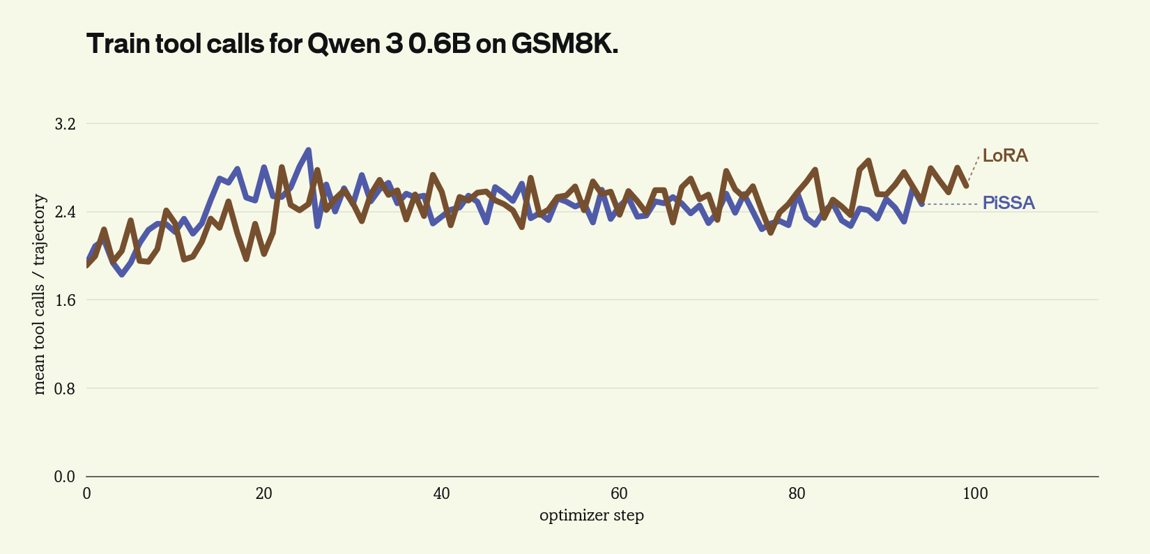
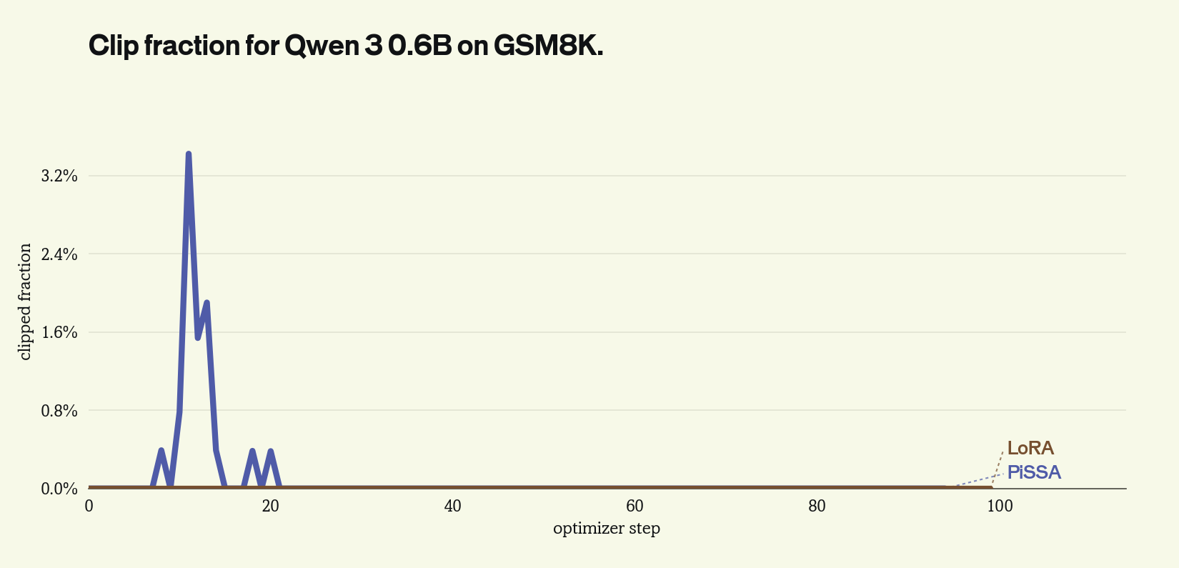
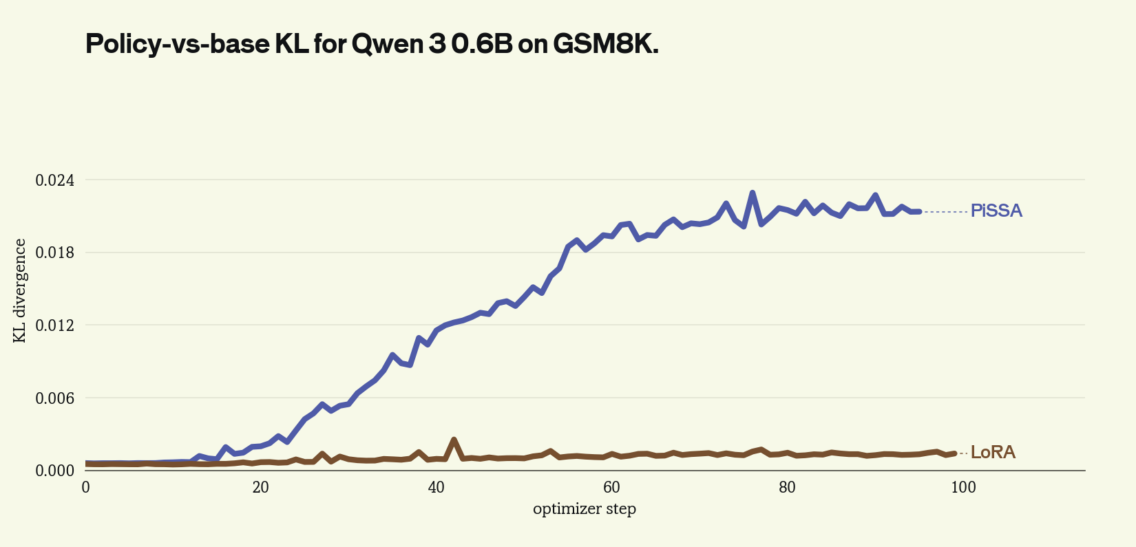
Mechanism panels for Qwen 3 0.6B on GSM8K, aligned over optimizer step: Frobenius distance traveled by the weights, KL divergence from the base policy, clipped token fraction, and tool calls per trajectory. Both arms use rank 32, the same data, the same seed, and a learning rate of 3e-6.

Qwen3 0.6B effective weight movement on GSM8K — Figure 10. Effective weight movement for Qwen 3 0.6B on GSM8K.

Qwen3 0.6B tool calls per trajectory on GSM8K — Figure 11. Train tool calls for Qwen 3 0.6B on GSM8K.

Qwen3 0.6B clipped token fraction on GSM8K — Figure 12. Clip fraction for Qwen 3 0.6B on GSM8K.

Qwen3 0.6B policy divergence from the base model on GSM8K — Figure 13. Policy-vs-base KL for Qwen 3 0.6B on GSM8K.

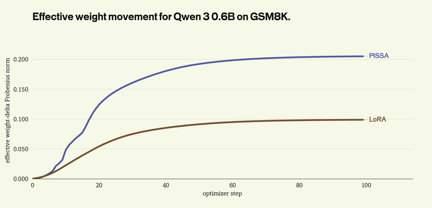
We examine the Frobenius distance between the original and post-trained weight matrices, which is the square root of the summed squared differences between the entries of $W$ and $W'$ :

d(W, W') = \sqrt{\sum_i \sum_j |W_{ij}-W'_{ij}|^2}.

This is equivalent to the straight line distance between the two weight matrices if each was rolled out into a 1-dimensional vector. Over 100 gradient steps, PiSSA moves the Qwen3-0.6B weights a Frobenius distance of 0.21, while LoRA moves 0.10, about half as far.

The policy moves with the weights. To quantify this, we compute the KL divergence $\text{KL}(\text{post-trained}\|\text{base})$ between the trained policy and the base model on the training rollouts. For LoRA, the KL stays relatively flat throughout training and ends at 0.001. However, for PiSSA, it ends at 0.021, twenty times higher.

PiSSA moves the weights further, and also moves the resulting policy further from the base policy. To understand why, notice that by derivative product rule, the gradient update to the low-rank adapter is:

d(AB) = (dA)B + A(dB).

Standard LoRA starts with $B = \mathbf{0}$ . The first term vanishes, and the second passes through a random $A$ . PiSSA starts with both factors aligned with the top singular directions, so both terms can contribute from the first step. When downstream task gradients align with these directions, PiSSA can changes the weights more per optimizer step early in training.

The larger KL divergence corresponds to a more verbose policy. Both arms start near 1.1k output tokens per trajectory. PiSSA rises to 3.6k while LoRA stays at 1.3k. On GSM8K, the added tokens mostly show up as longer reasoning traces. Both runs are reasonably stable: PiSSA only clips a brief burst of tokens early in training, and the LoRA run's clipped fraction stays at zero.

At a fixed learning rate, principal initialization moves the weights and the policy further per optimizer step than random initialization, and that movement arrives as longer reasoning traces and higher accuracy. Our experiments here do not isolate whether the gain comes from the larger effective step or from the specific directions the principal subspace selects. Initialization schemes that start both factors nonzero without the principal subspace would separate the two; we leave that comparison to future work.

Limitations and Future Work

Given additional time and compute, we would strengthen these results with a hyperparameter sweep across learning rates and regularization terms (e.g., KL regularization, advantage clipping, gradient clipping, etc). A common critique of PiSSA and other SVD-based initializations is that they are less stable [5].

We note that our work excludes a variety of other initialization schemes, VeRA, DoRA, QLoRA, etc, as well as simple ideas such as [8] which show that simply swapping $A \sim \mathcal{N}(0,\sigma^2), \; B = \mathbf{0}$ to $A = \mathbf{0}, \;B \sim \mathcal{N}(0,\sigma^2)$ can result in better training stability. Concurrent work proposes LoRA-RLPO and LoRA-RLMO initializations that use an SVD initialization for $A$ but zero out $B$ [5].

The MiLoRA initialization is especially relevant to the theoretical ideas posed in this blog. While PiSSA selects the top k ranks of each weight matrix’s SVD as the low-rank adapter, MiLoRA selects the bottom k ranks [9]. In supervised fine-tuning, this initialization aims to prevents catastrophic forgetting, since the updated directions are orthogonal to the directions stretched most during pretraining.

There are ample open directions left for optimizing LoRA initializations for RL. Our work aims to demonstrate that initialization schemes are important and scalable for parameter-efficient RL, and we are excited to continue exploring new research ideas in this direction. In particular, we note that selecting top/bottom SVD ranks aligns the LoRA initialization to the pretraining task distribution. Instead, the best initialization might be task-specific and selected to align with activations or gradients on (a sample from) the target downstream task.

We also note that our current experiments are limited to dense models. Please see Contributions to SkyRL for more discussion on added challenges with PiSSA for MoEs, and our current progress in that direction.

Looking farther out, we’re also curious whether midtraining can condition base models to be more post-trainable. For example, favoring wide minima in the pretraining loss landscape [6] and retaining many active learnable directions [7] might result in better post-trainability, independent of initialization. There is plenty of science left to do in parameter-efficient fine-tuning, and if you’re excited about this kind of work, consider joining us!

Technical contributions to SkyRL

As part of this blog, we are releasing PiSSA support in SkyRL. You can view the changes at SkyRL#2069, including example scripts to reproduce the cheap Qwen3-0.6B results.

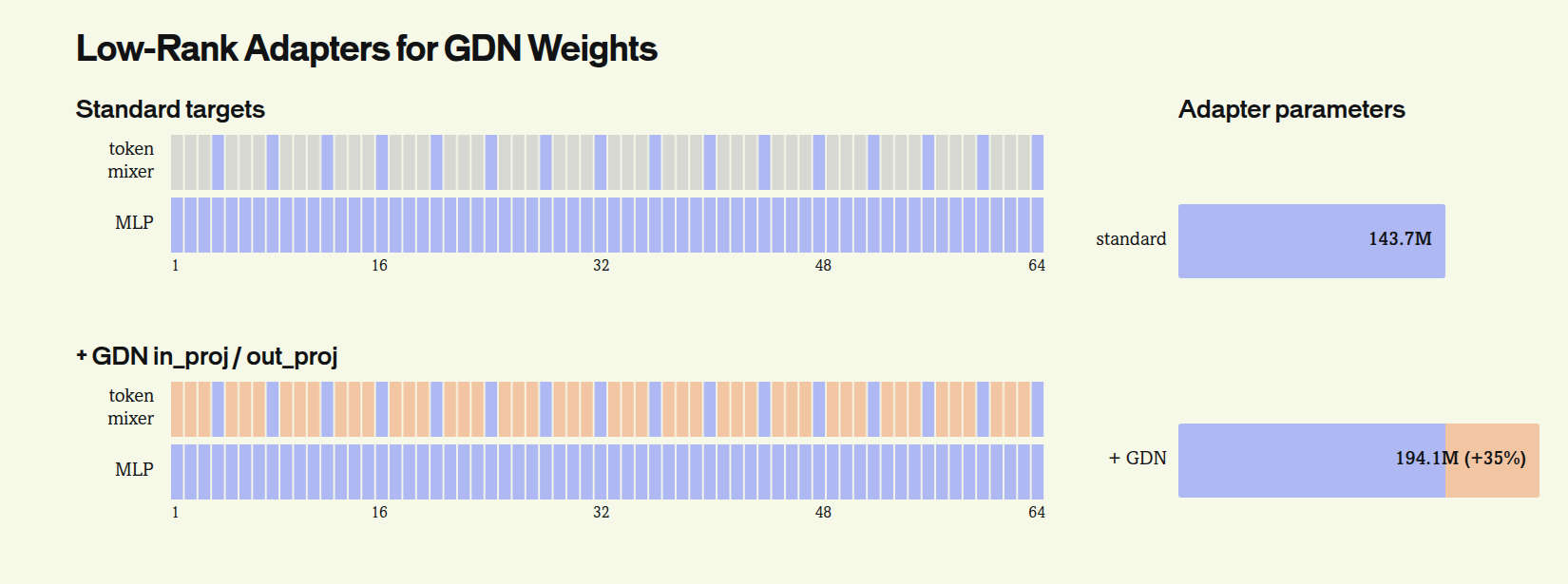
Here, we highlight two interesting technical challenges with scaling PiSSA to modern architectures. During our initial experiments with Qwen3.6-27B, we noticed that most of the attention layers were frozen with no adapters. These layers used Gated DeltaNet (GDN) linear attention which replaces the traditional $W_Q,W_K,W_V$ with $W_{in},W_{out}$ matrices [10]. We added low-rank adapters to these matrices as well.

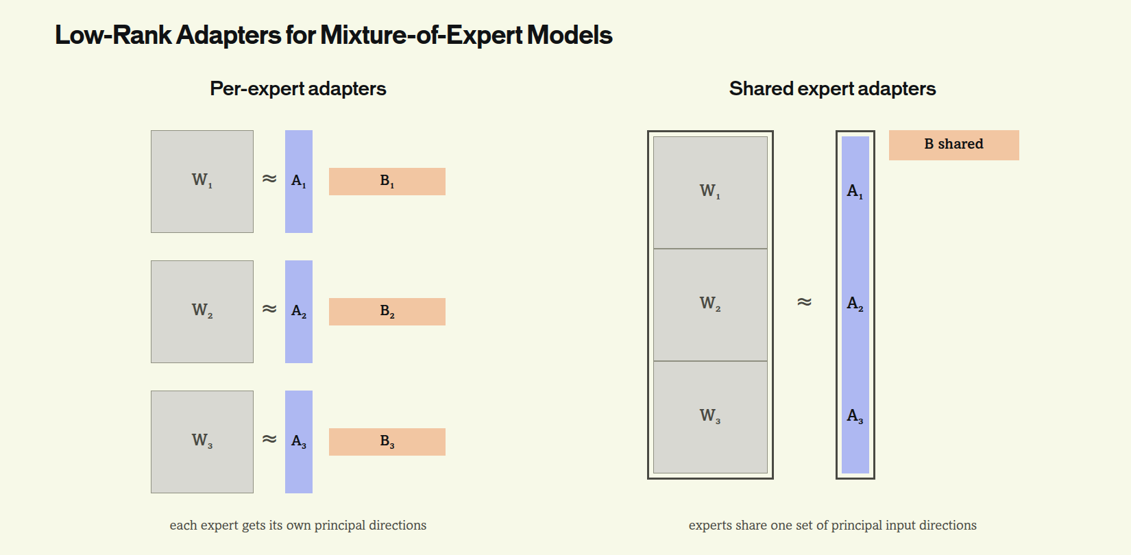
Qwen3.6 27B adapter parameters with and without GDN projections — Figure 14. Adding low-rank adapters to the GDN matrices grows the Qwen3.6-27B trainable parameter count by 35%, but the adapters remain only 0.72% of the base model.

As noted earlier, this blog focuses on dense architectures. However, we also add support for MoE architectures, and validated them on Qwen3-30B-A3B. By default, SkyRL uses shared-expert LoRA: all experts share a single $B$ matrix. This weight tying saves parameters, and in practice, does not affect LoRA training [11].

However, when doing SVD, this means that some experts may be overrepresented in the top $r$ ranks whereas others may be mostly ignored. We turn expert-sharing off for PiSSA, but note that this might not always be practical.

Shared and independent expert adapter parameter counts — Figure 15. For GLM 5.2 (700B total parameters), training rank-32 LoRA adapters with shared-expert adapters use 149M parameters, but disabling expert sharing increases this to 11B parameters.

Citations

[1] Hu, E. J., Shen, Y., Wallis, P., Allen-Zhu, Z., Li, Y., Wang, S., Wang, L., & Chen, W. (2021). LoRA: Low-rank adaptation of large language models. arXiv. https://doi.org/10.48550/arXiv.2106.09685

[2] Schulman, J., & Thinking Machines Lab. (2025, September 29). LoRA without regret. Thinking Machines Lab. https://thinkingmachines.ai/blog/lora/

[3] Biderman, D., Portes, J., Gonzalez Ortiz, J. J., Paul, M., Greengard, P., Jennings, C., King, D., Havens, S., Chiley, V., Frankle, J., Blakeney, C., & Cunningham, J. P. (2024). LoRA learns less and forgets less. arXiv. https://doi.org/10.48550/arXiv.2405.09673

[4] Meng, F., Wang, Z., & Zhang, M. (2024). PiSSA: Principal singular values and singular vectors adaptation of large language models. arXiv. https://doi.org/10.48550/arXiv.2404.02948

[5] Zhang, R., Zhu, J., Zhu, H., & Shi, L. (2026). Geometry-preserving orthonormal initialization for low-rank adaptation in RLVR. arXiv. https://doi.org/10.48550/arXiv.2606.31813

[6] Watts, I., Li, C., Goyal, S., Springer, J. M., & Raghunathan, A. (2026). Sharpness-aware pretraining mitigates catastrophic forgetting. arXiv. https://doi.org/10.48550/arXiv.2605.02105

[7] Prakash, A., He, N., Guo, K., Tiwari, S., Tao, R. Y., Serapio, T., Greenwald, A., & Konidaris, G. (2025). Spectral collapse drives loss of plasticity in deep continual learning. arXiv. https://doi.org/10.48550/arXiv.2509.22335

[8] Hayou, S., Ghosh, N., & Yu, B. (2024). The impact of initialization on LoRA finetuning dynamics. arXiv. https://doi.org/10.48550/arXiv.2406.08447

[9] Wang, H., Li, Y., Wang, S., Chen, G., & Chen, Y. (2024). MiLoRA: Harnessing minor singular components for parameter-efficient LLM finetuning. arXiv. https://doi.org/10.48550/arXiv.2406.09044

[10] Yang, S., Kautz, J., & Hatamizadeh, A. (2024). Gated Delta networks: Improving Mamba2 with Delta rule. arXiv. https://doi.org/10.48550/arXiv.2412.06464

[11] NVIDIA. (2026, January 13). A comparison of performant and canonical LoRA variants. NVIDIA NeMo Framework User Guide. https://docs.nvidia.com/nemo-framework/user-guide/25.07/sft_peft/canonical_lora.html

[12] Qwen Team. (2025). Qwen3 technical report. arXiv. https://doi.org/10.48550/arXiv.2505.09388

Acknowledgements

We thank Chuck Tang for his technical guidance and advice with implementing and testing PiSSA, Eric Tang for his invaluable help with SkyRL implementation and testing, and Arjun Karanam and Michael Elabd for their technical leadership and feedback on early drafts of this post.